
Algorithmic Composition: A Gentle Introduction to Music Composition Using Common LISP and Common Music
Skip other details (including permanent urls, DOI, citation information): This work is protected by copyright and may be linked to without seeking permission. Permission must be received for subsequent distribution in print or electronically. Please contact mpub-help@umich.edu for more information.
For more information, read Michigan Publishing's access and usage policy.
Title Page
Title // Algorithmic composition: a gentle introduction to music composition using common LISP and common music
Author // Mary Simoni
Series // SPO Scholarly Monograph Series
Publisher // The Scholarly Publishing Office, The University of Michigan, University Library
Place of Publication // Ann Arbor, Michigan
Date of Publication // 2003
Copyright C 2003 by the Regents of the University of Michigan. All rights reserved. No part of this book may be reproduced without permission of the authors. Authors retain the copyright to their individual works. The Regents of the University of Michigan David A. Brandon, Ann Arbor; Laurence B. Deitch, Bingham Farms; Olivia P. Maynard, Goodrich; Rebecca McGowan, Ann Arbor; Andrea Fischer Newman, Ann Arbor; Andrew C. Richner, Grosse Pointe Park S. Martin Taylor, Gross Pointe Farms; Katherine E. White, Ann Arbor; Mary Sue Coleman, ex officio Please contact The Scholarly Publishing Office at the University of Michigan, University Library for permission information: Scholarly Publishing Office 300 Hatcher N Ann Arbor, MI 48109 lib.spo@umich.edu
The University of Michigan University Library through its Scholarly Publishing Office is committed to providing academic publishing services that are responsive to the needs of both producers and users, that foster a sustainable economic model for academic publishing, and that support institutional control of intellectual assets. The Scholarly Publishing Office seeks to disseminate high-quality, cost-effective scholarly content through both print and electronic publishing. Information about the Scholarly Publishing Office can be found at http://spo.umdl.umich.edu.
Acknowledgements
This book would not have been possible if it were not been for the dedicated work of Heinrich (Rick) Taube. Rick has worked tirelessly, with the support of Tobias Kunze, on the development of Common Music. Whenever there was an issue regarding some aspect of Common Music, Rick or Tobias would quickly tackle the technical problems to make the software more responsive.
I also acknowledge the work of David S. Touretzky for his influential book, "Common LISP: A Gentle Introduction to Symbolic Computation." Although this book is no longer in print, it has been an invaluable teaching tool and reference for myself and my students. Touretzky's emphasis on simplicity has opened the door of algorithmic composition to many music composition students.
I would also like to thank my students who carefully reviewed this book prior to publication: Todd Bauer, Nathaniel Cartier, Michael Chiaburu, Hiroko Fukudo, Matthew Gill, Colin Meek, Christopher Peck, Nathan Proulx, Jennifer Remington, Christopher Rozell, Stephen Alex Ruthmann, Michael Vartanian, and John Woodruff. Their thoughtful comments and contributions have increased the accessibility and relevance of the content.
Preface
This book is about learning to compose music using the programming language Common LISP and the compositional environment Common Music developed by Heinrich Taube.
The motivation for writing this book comes from several years of teaching music and engineering students the fundamentals of algorithmic composition. Algorithmic composition, for the purposes of this book, is defined as the use of computers to implement procedures that result in the generation of music. The idea of applying algorithms during the composition of music is pervasive throughout music history. The intent of this book is to give the reader the fundamentals of Common LISP and Common Music accompanied by examples of algorithmically based compositions. Although not every aspect of Common LISP and Common Music are covered in this book, the reader will be well equipped to develop their own algorithms for composition.
As I wrote this book, I kept the needs of several kinds of readers foremost in mind:
Musicians - These readers know the fundamentals of tonal music theory and have had formal instruction in music performance and composition. These readers may or may not have studied a programming language.
Engineers - These readers have significant experience in designing and implementing algorithms but not necessarily for music. They have some knowledge of tonal music theory but have not likely had formal instruction in music performance or composition.
Researchers - These readers have experience in both music and engineering and are interested in quickly and efficiently learning the fundamentals of Common Music.
This book is organized into three sections. Section I, comprised of Chapters 1 through 4, introduces the fundamentals of programming in Common LISP and Common Music. Section I also includes a historical survey of algorithmic composition. Section II, comprised of Chapters 5 through 14, is the core content of the book. These chapters contain detailed information on the integration of Common LISP and Common Music with an emphasis on music composition. Some readers may choose to reverse their study of recursion (Chapters 13) and iteration (Chapter 14). Readers with less programming experience generally find it easier to understand recursion if they have first studied iteration. Chapters 13 and 14 have many parallel examples designed to help the reader understand the differences between iteration and recursion through direct comparison. Section III, comprised of Chapters 15 and 16, may be regarded as advanced topics in algorithmic composition.
The reader may need the assistance of an instructor or Common LISP documentation for implementation-specific information. Common LISP implementations have their own commands or user interface. The reader is well advised to make sure their implementation of Common LISP includes an editor.
I am very much in gratitude to the University of Michigan School of Music for their excellent music technology facilities, technical staff, and loyal support of my work.
Chapter 1: Introduction
This book integrates three subject areas: Common LISP, Common Music, and algorithmic composition. The purpose of combining these three subjects into one book is to assist readers who are interested in composing music using computers. The author assumes the reader has very little experience with Common LISP or Common Music. For this reason, usage and syntax of Common LISP and Common Music are explained through numerous carefully documented examples. The author assumes the reader has an understanding of tonal music theory and MIDI (The Musical Instrument Digital Interface) [IMA, 1983]. The majority of the examples in this book and the accompanying compact disc use MIDI.
Many wonderful compositions have been written over the years using Common LISP and Common Music. By making the details of how to use Common Music more approachable, the author hopes more people will be enticed to explore the potential of algorithmic composition.
1.1 Common LISP
The programming language LISP derives its name from List Processing [Winston, 1989]. Common LISP was developed in 1956 by artificial intelligence researchers Allen Newell, J.C. Shaw, and Herbert Simon [Touretzky, 1990]. Since the early days of LISP, researchers have discovered the power of LISP's processing capabilities for music. Music, a time-based art form, oftentimes is conceived as a succession of events. The events may be a series of pitches, articulation patterns, or a succession of rhythms. Figure 1.1.1 depicts a pitch series that is accompanied by a list representation of that series. Each item in the list representation is called an element.
Figure 1.1.1
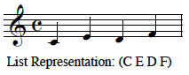
Once musical events are described as elements of a list, Common LISP functions may be applied to each element of the list to transform the elements. One such example might be to transpose every element of the list in Figure 1.1.1 up a major second returning the list (D F-sharp E G). Beginning with Chapter 3, we will learn how to use Common LISP to build programs that transform musical data.
1.2 Common Music
Common Music is an extensible programming environment for computer-based composition. The development of Common Music began in 1989 by Heinrich Taube [Taube, 1989]. After several years of continuous evolution, Common Music was awarded first prize in the computer-assisted composition category at the 1er Concours International de Logiciels Musicaux in Bourges, France.
Common Music is implemented in Common LISP and the Common LISP Object System [Keene, 1989]. Common Music's command line interface is called Stella. Common Music runs on Macintosh, Windows, and UNIX platforms. The software and accompanying electronic documentation is available as freeware at a number of internet sites [Taube, 2000]. Common Music requires that Common LISP be installed on your computer system. You may think of Figure 1.2.1 when conceptualizing the software layers required by Common Music.
Figure 1.2.1: The software layers required by Common Music

Common Music works in conjunction with a number of other protocols and applications for the display and realization of music. For example, it is possible to use MIDI for both input and output to Common Music. MIDI input and output requires that Common Music communicates with your system's MIDI driver. Appendix A describes how to configure Common Music for MIDI input and output using the OMS (Open Music System) MIDI driver. The majority of examples in this book and accompanying compact disc use MIDI.
Another way to use Common Music is in conjunction with Csound, sound synthesis software developed by Vercoe and Karstens. Common Music outputs parameter values to a Csound scorefile that is referenced by a Csound orchestra file. Appendix B describes how to configure Common Music to output data using the Csound scorefile format [Boulanger, 1999].
Common Music outputs data to a number of other sound synthesis applications including Common Lisp Music [Schottstaedt, 1991], Cmix [Lansky, 1990], and Cmusic [Moore, 1990] as well as music notation software such as Common Music Notation developed by Schottstaedt.
1.3 Algorithmic Composition
An algorithm is defined as a set of rules or a sequence of operations designed to accomplish some task or solve a problem. Human beings are very good at designing and implementing algorithms. From getting dressed in the morning to cooking dinner, we are continuously developing algorithms to solve life's everyday problems.
Gareth Loy describes criteria for determining the validity of an algorithm [Loy, 1989]. An algorithm must have a finite number of steps; have both input to and output from the algorithm; yield a result in a finite period of time; and have a precise definition for each step of the algorithm. Donald Knuth explains that there are also aesthetic criteria for the evaluation an algorithm [Knuth, 1973]. These aesthetic criteria include simplicity, parsimony, elegance, and tractability. Ideally, algorithms should strive to meet the criteria outlined by Loy and Knuth.
Composition is the process of creating a musical work [Apel, 1979]. The term composition literally means to "put together" parts into a unified whole. The process of composing music is oftentimes characterized by trial and error. The composer tries something, listens, and determines if revisions are necessary. The composer is continually evaluating the effectiveness of a part in relation to the whole.
We combine the terms algorithm and composition to derive the term algorithmic composition. Algorithmic composition, in the simplest sense, is when a composer uses an algorithm to put together a piece of music. Since the mid-twentieth century, the computer has become a key partner in implementing algorithms that generate music. Because of the increased role of the computer in the compositional process, algorithmic composition has come to mean the use of computers to implement compositional procedures that result in the generation of music.
1.4 Additional References
Although this book provides you with the fundamentals of algorithmic composition using Common LISP and Common Music, you may wish to augment your reading with additional references. Two excellent Common LISP references include, "LISP" by Patrick Henry Winston and Bertold Klaus Paul Horn [Winston, 1989] and "Common LISP - The Language" by Guy L. Steele [Steele, 1990]. Common Music is accompanied by voluminous electronic documentation, much of it in HTML. The Common Music Dictionary , available on the accompanying CD and the Common Music FTP site [Taube, 2000], is a quick reference covering most aspects of Common Music. For detailed information on MIDI, consult the MIDI Specification and supporting documents published by the International MIDI Association [IMA, 1983] or a textbook on MIDI such as "MIDI: A Comprehensive Introduction" by Joseph Rothstein [Rothstein, 1992]. For additional information on strategies for algorithmic composition, refer to Chapter 19 of "The Computer Music Tutorial" by Curtis Roads [Roads, 1996] or Chapter 11 of "Computer Music: Synthesis, Composition, and Performance" by Charles Dodge and Thomas Jerse [Dodge, 1997].
Chapter 2: The History and Philosophy of Algorithmic Composition
In Chapter 1, we defined algorithmic composition as the use of a rule or procedure to put together a piece of music. This chapter will give you a broader understanding of algorithmic composition, how algorithms have been used throughout music history, and an introduction to the aesthetic issues of algorithmic composition.
2.1 The Process of Algorithmic Composition
A very simple example of using a procedure to generate a piece of music is to use a 12-sided die (numbered 1-12) to determine the order of pitches in a composition. An association, or mapping is made to correlate each pitch in a twelve-tone equal tempered scale with each number on the die. Figure 2.1.1 demonstrates the mapping of pitches to numbers.
Figure 2.1.1

Let's say that we decide to roll the die six times. Our six tosses return the numbers 2, 5, 3, 9, 3, and 12. The music that results from our roll of the die is found in Figure 2.1.2.
Figure 2.1.2

Can such a simple algorithm produce interesting music? How do we determine the other aspects of the composition such as rhythm, timbre, loudness, register, etc.? These questions have been explored by composers throughout music history.
2.2 A Brief History of Algorithmic Processes Applied to Music Composition
The Greek philosopher, mathematician, and music theorist Pythagoras (ca. 500 B.C.) documented the relationship between music and mathematics that laid the foundation for our modern study of music theory and acoustics. The Greeks believed that the understanding of numbers was key to understanding the universe. Their educational system, the quadrivium, was based on the study music, arithmetic, geometry, and astronomy. Although we have numerous treatises on music theory dating from Greek antiquity, the Greeks left no clues if mathematical procedures were applied to the composition of music.
Over a thousand years later, the work of music theorists such as Guido d'Arezzo established the framework for our conventional system of music notation. His system employed a staff accompanied by a clef making it possible for a composer to notate a score so that it could be performed by someone other than the composer. Prior to the development of the score, music was learned by rote and generally improvised and embellished by the performing musician. By the thirteenth century, formalized music composition began to replace improvisation and the role of composer and performer became increasingly distinct.
The music theorist Franco of Cologne established rules for the time values of single notes, ligatures, and rests in his treatise Arts canus mensurabilis (ca. 1250). By the early fourteenth century, composers began to treat rhythm independently of pitch and text. French composers of the ars nova , such as Phillipe de Vitry and Guillaume de Machaut, used isorhythm as a means of unifying their compositions. Iso means "same" so isorhythm means literally "same rhythm." Isorhythm is the practice of mapping a rhythmic sequence, named the talea , onto a pitch sequence called the color . Figure 2.2.1 depicts the talea from the motet De bon espoir-Puisque la douce-Speravi by Guillaume de Machaut.
Figure 2.2.1: Talea of the isorhythmic motet De bon espoir-Puisque la douce-Speravi by Guillaume de Machaut

The next figure shows the color of the same motet.
Figure 2.2.2: Color of the isorhythmic motet De bon espoir-Puisque la douce-Speravi by Guillaume de Machaut.

The tenor of De bon espoir-Puisque la douce-Speravi was derived by mapping the color onto the talea as shown in Figure 2.2.3.
Figure 2.2.3: The tenor of De bon espoir-Puisque la douce-Speravi by Guillaume de Machaut

Phillipe de Vitry used a palindrome in the construction the talea for his isorhythmic motet Garrit gallus - In nova fert. A palindrome is a pattern that reads the same forwards as it does backwards. Figure 2.2.4 shows the organization of the palindrome by measure. Measure 1 compares to measure 9, measure 2 compares to measure 8, etc.
Figure 2.2.4: The talea of Garrit gallus - In nova fert by Phillipe de Vitry

The Renaissance period witnessed the rise of polyphonic sacred and secular musical forms. By the Baroque Period (1600-1750), highly developed contrapuntal forms such as the canon and fugue flourished. One of the great masters of contrapuntal forms was Johann Sebastian Bach. During the final years of his life, J.S. Bach composed such didactic contrapuntal works such as the Musical Offering and The Art of the Fugue [Bach, 1752]. The Art of the Fugue is a brilliant pedagogical tool for the study of counterpoint that systematically documents the procedure of fugal and canonic composition.
The canon is a highly procedural contrapuntal form. The composer begins with a melody, called the leader, which is strictly followed at a delayed time interval by another voice, called the follower. Sometimes, the follower may present a variation of the leader through transposition, augmentation, or inversion. Figure 2.2.5 shows an excerpt from The Art of the Fugue by J.S. Bach that is a canon in both augmentation and inversion.
Figure 2.2.5: Canone I from The Art of the Fugue by J.S. Bach

In the final fugue of The Art of the Fugue, Fuga XV , J.S. Bach uses his own name,B-A-C-H, as the subject of the fugue: B-flat, A, C, and H. (H is the German letter for B). His name is embedded in one of the most masterful contrapuntal works of all time.
Figure 2.2.6: Excerpt from Fuga XV from The Art of the Fugue by J.S. Bach

One of the most often cited examples of algorithmic music in the Classical Period (1750-1827) is Musikalisches Würfelspiel by Wolfgang Amadeus Mozart (1756-1791). In this composition, Mozart composed discrete musical excerpts that could be combined to form a waltz. The order of musical excerpts was determined by rolling two six-sided dice. The person assembling the waltz would refer to a table created by Mozart that showed which music should be used for the values of 2-12 on the dice.
Romanticism pushed the harmonic vocabulary into the extreme use of chromaticism. After Richard Wagner (1813-1883), there was very little a composer could do that would be considered novel using tonal music theory. Arnold Schoenberg, and his pupils Anton Webern and Alban Berg, established new procedures for composition called serial composition .
In serial composition, the composer works with a series of twelve chromatic tones of equal importance. In strict serial composition, no tone may be repeated until all twelve have been used. The total number of twelve-note series is 479,001,600 [Brindle, 1969] which greatly expands the melodic and harmonic vocabulary of the late Romantic period. Because of the equal importance of the twelve chromatic tones, serial composition eroded tonality and gave rise to atonality.
Algorithmic procedures lend themselves well to serial composition. To introduce variation into a serial composition, the composer may use permutations of the tone row derived from transposition, inversion, retrograde, or retrograde inversion of the row. Figure 2.2.7 shows the tone row used by Alban Berg in the Lyric Suite for string quartet composed in 1926.
Figure 2.2.7: The tone row for the Lyric Suite by Alban Berg

Figure 2.2.8 shows a matrix that was constructed based on the tone row from Alban Berg's Lyric Suite . The Rows are numbered 1-12 and the Columns are labeled A-L. The original form of the tone row is found in Row 1, Columns A-L, reading from left to right. The retrograde form of the tone row is found by reading Row 1, Columns A-L, reading from right to left. The inversion of the tone row is found in Column A reading Row 1 to Row 12 and the retrograde inversion is found in Column A reading from Row 12 to Row 1. Each Row and Column is further labeled with T followed by a value in the range 0-11. The T stands for transposition and the number is the level of transposition measured in half steps from the original tone row. For example, T5 means the tone row has been transposed up five half steps from the original form (e.g. a Perfect Fourth).
Figure 2.2.8: Tone Row Matrix for Alban Berg's Lyric Suite

About the same time Alban Berg completed the Lyric Suite , Iannis Xenakis (1922-) began to make his way in the world. Xenakis received an engineering degree from the Athens Polytechnic School and studied music composition with Honegger, Milhaud, and Messiaen and architecture with Le Corbusier. Xenakis was keenly interested in the application of mathematics to music composition. In 1966, Xenakis founded the School of Mathematical and Automated Music in Paris. His music is described as stochastic music meaning he uses probability theory in the selection of musical parameters. Xenakis exploited probability theory in his search for new musical form and structure. One of Xenakis' well-known works, Pithoprakta (1955-56), creates dense sound masses determined by probabilistic methods.
The music of Karlheinz Stockhausen (1928-) stands in sharp contrast to that of Iannis Xenakis. Stockhausen developed serial composition to its extreme by not only applying serial methods to pitch, but also rhythm, dynamics, timbre, and density. Stockhausen was influenced by the German philosopher Hegel and his doctrine on the unity of opposites. Stockhausen applied Hegelian philosophy by using calculations to pre-compose his music while integrating chance operations into the performance. A stunning example of his work is the Klavierstück X1 (1956) composed for piano. The score, measuring about thirty-seven inches by twenty-one inches, consists of nineteen carefully composed segments that the pianist performs in whatever order his or her eye happens to fall upon the score. Stockhausen employed chance operations similar to those explored by Mozart in his Musikalisches Würfelspiel almost two hundred years earlier.
About the same time Stockhausen composed the Klavierstück X1, Lejaren Hiller and Leonard Issaacson were preparing to significantly alter the course of music history. Ada Augusta, Countess of Lovelace worked with Charles Babbage on the development of a mechanical computer called the Analytical Engine. In 1842, she described the use of the computer in the creation of music and foretold the era of computer-assisted composition heralded by Hiller and Isaacson:
"The operating mechanism [of the Analytical Engine]. . .might act upon other things. . . whose mutual fundamental relations could be expressed by those of the abstract science of operations, and which should be also susceptible of adaptations to the act ion of the operating notation and mechanism of the Engine. Supposing, for instance, that the fundamental relations of pitched sounds in the science of harmony and of musical composition were susceptible of such expression and adaptations, the Engine might compose and elaborate scientific pieces of music of any degree of complexity or extent." [Roads, 1996]
It was 1957 when Lejaren Hiller and Leonard Isaacson programmed the ILLIAC computer at the University of Illinois to algorithmically generate music. The output of their software created The ILLIAC Suite scored for string quartet. The work of Hiller and Issaacson is documented in the book "Experimental Music." [Hiller, 1959]. By 1962, Xenakis began to use the computer to assist in the calculations for his compositions Amorsima-Morsima and Strategie, Jeu pour deux orchestres.
John Cage (1912-1992) was a self-declared indeterminist. Cage integrated Eastern philosophies, especially Zen Buddhism, and the I Ching Book of Changes, into his compositions. A landmark collaboration between Cage and Hiller resulted in the multi-media composition HPSCHD (1967-1969), The composition uses computer print outs, excerpts of traditional music, and visual elements depicting space and rocket technology. The traditional music is derived from Mozart's Musikalisches Würfelspiel and his piano Sonatas. Cage's statement, "it is the machine that will help us to know whether we understand our own thinking processes," demonstrates his philosophical comradeship with Lejaren Hiller. HPSCHD requires up to seven harpsichords and fifty-one electronic tapes that are combined in any possible way to achieve unique performances. The composition received its world premiere before an audience of nine thousand at the University of Illinois on May 16, 1969. The performance included all seven harpsichords, fifty-one computer-generated tapes, eighty slide projectors, and seven film projectors.
For over two thousand years, composers have used algorithms to assist in the creation of new works. Algorithms for music composition have evolved into several categories: aleatoric (or chance) methods [e.g. Cage]; determinacy [e.g. Schoenberg, Webern, and Berg]; and stochastic (or probabilistic) methods [e.g. Xenakis and Hiller]. Composers are applying not only mathematical models but also biological paradigms to the creation of music. Since almost any process may be modeled using a computer, almost any model may be used for music composition.
The principle questions facing composers who use algorithmic processes are rooted in aesthetics and philosophy. Why use algorithms in the composition of music? What is more important- the algorithm or the composition? How does a composer or listener decide if an algorithmic composition is successful?
2.3 Aesthetics of Algorithmic Composition
Aesthetics is a branch of philosophy that describes the theories and forms of beauty in the fine arts. It is our unique set of experiences, and our perception of those experiences, that shape our personal aesthetic. Our personal aesthetic is integrally intertwined with our personality as an artist. Each work of art is some manifestation of the artist's aesthetic.
In Chapter 1, we discussed Knuth's principles for determining the aesthetic merit of an algorithm. How do we decide if a composition that uses algorithms has aesthetic merit?
To answer this question, one must separate the process of composition from the product of composition, e.g. the music. Some algorithmic composers would argue that the aesthetic merit of an algorithmic composition should be based solely on the algorithm used to create the music. Other composers assert that both the algorithms used to create the composition and the composition itself should be assessed when determining aesthetic merit. There are still others who would argue that the algorithms used in algorithmic composition are simply a means to an end and for that reason, the algorithms themselves are not worthy of artistic scrutiny. These composers may believe that their success or failure as a composer is based on the listener's response, and therefore they have the right to throw away or modify the output of an algorithm to achieve their aesthetic goal.
All of these responses to the process and product of algorithmic composition are valid as each view is simply a manifestation of a personal aesthetic. Unfortunately, composers of algorithmic music have not been formally surveyed regarding their views on the aesthetics of algorithmic composition so we do not know how many composers fall into which category at any given time or if there are more categories to consider.
In the absence of a formal survey, we let the repertoire of algorithmic composition speak for itself. In reviewing algorithmic processes throughout the twentieth century, the number of compositions that are supported by documented algorithms are dwarfed by those that are not. In fact, when asking composers to provide algorithms accompanied by software implementation for this book, many composers confided that their code is not up to Knuth's standards of simplicity, elegance, parsimony, and tractability. With rapid advances in automated music composition systems, and the tendency to embed the process in a technology, it is inherently more difficult for the process to survive than it is the product.
A group of visual and sonic artists developed their own criteria for determining the aesthetic merit of electronic art, including computer music [Mandelbrojt, 1999]. These artists felt the criteria should be based on the poetic quality of the artist's vision; a successful relationship between the artist's idea and its realization, especially when the idea cannot be materialized through simpler traditional means; the efficiency with which the artist's idea is conveyed; and the originality of the idea or its realization. The evaluation of each of these criteria is not simply a "yes" or "no" as in the case of Knuth's criteria. On the contrary, the criteria summarized by Mandelbrojt require a graded continuum for each criterion to render an aesthetic judgement about a work. These criteria also presuppose that the person performing the evaluation knows something of the artist's intent. Unfortunately, such is not always the case.
Algorithmic composers need aesthetic criteria that are neither as limiting as Knuth's nor as assumptive as those described by Mandelbrojt. Composers of algorithmic music are obliged to carefully examine the quality of their artistic idea and the efficiency in which that idea is presented. The composer must create a successful relationship between the artistic idea and the technological medium in which they work. The work must demonstrate originality or significant refinement of an existing idea and maintain the highest quality of technical production.
2.4 Suggested Listening
Garrit gallus - In nova fert by Phillipe de Vitry
Musical Offering and The Art of the Fugue by J.S. Bach
Musikalisches Würfelspiel by Wolfgang Amadeus Mozart
Lyric Suite by Alban Berg
Klavierstück XI by Karlheinz Stockhausen
The ILLIAC Suite by Lejaren Hiller and Leonard Isaacson
Amorsima-Morsima and Strategie, Jeu pour deux orchestres by Iannis Xenakis
HPSCHD by John Cage
Chapter 3: Introduction to Common LISP
Chapter 3 introduces you to the fundamentals of Common LISP and programming in LISP. You will learn about some of the various data types that Common LISP supports and many of its built-in functions called primitives . You will learn how to write your own functions and become familiar with typical error messages.
3.1 Data and Functions
Data is information. Common LISP supports several data types including numbers, symbols, and lists.
Numbers may take several forms including integers or whole numbers, ratios or fractions, and floating point numbers.
Another data type in Common LISP is a symbol. Symbols look like words and may contain any combination of letters and numbers along with some special characters like the hyphen (-) or underscore (_).
There are two special symbols in Common LISP: T and NIL. T represents TRUE or YES and NIL represents FALSE, NO, or NOTHING.
Another data type in Common LISP is a string. A string is a sequence of characters enclosed in double quotes.
A very important Common LISP data type is the list. Lists are at the heart of programming in LISP, which derived its name from LISt Processing. A list is a collection of one or more things enclosed in parentheses. If the list includes more than one thing, they are space delimited. Each thing in the list is called an element. Therefore the list (C-MAJOR D-MAJOR F-MAJOR) has three elements and the list(+ 4.5 23/8 .0007 -23) has 5 elements.
Lists may be represented in the computer's memory as a chain of cons cells. You may think of a cons cell as having two parts. The left part is referred to as the CAR and the right part is referred to as the CDR. Each part of a cons cell has a pointer. The CAR pointer points to an element in a list and the CDR points to the next element in the list. Figure 3.1.1 is a cons cell representation of the list (C-MAJOR D-MAJOR F-MAJOR). Notice that the cons cell chain ends in NIL.
Figure 3.1.1

Lists that consist of one level of a cons cell chain are called a flat list .
When a list contains another list, it is referred to as a nested list . An example of a nested list is (C-MAJOR (C E G)). The top-level of the chain of cons cells contains two elements: the symbol C-MAJOR and the list (C E G). The next level down of the chain of cons cells contains three elements namely the symbols C, E, and G. Figure 3.1.2 is a cons cell representation of the nested list (C-MAJOR (C E G)).
Figure 3.1.2

Lists that have the same number of left parentheses and right parenthesis are called well-formed lists . Both (C-MAJOR D-MAJOR F-MAJOR) and (C-MAJOR (C E G)) are well-formed lists.
Now that we are familiar with some Common LISP data types, it's important to learn how these data types relate to each other. Both numbers and symbols are categorized as atoms. An atom is the smallest object that cannot be represented by a cons cell. A list, on the other hand, is a chain of cons cells. Atoms and lists form what are called symbolic expressions. Figure 3.1.3 gives an overview of some Common LISP data types.
Figure 3.1.3
Each particular instance of a data type is called an object. Therefore 78.3, MY-CHORD, and (C-MAJOR (C E G)) are all objects.
3.2 LISP Primitives
Functions operate on data. Functions allow us to process data to achieve a result. Common LISP functions may be categorized as either primitives or user-defined functions. You may think of functions as procedures that operate on data. Evaluating an expression is referred to as evaluating a form. A form is simply some Common LISP expression.
A primitive is a built-in function or simply put, a function that LISP already knows about. LISP has many primitives that operate on numbers, symbols, and lists.
LISP primitives that function on numbers include basic arithmetic operations such as addition, subtraction, multiplication, and division as well as more advanced arithmetic operations such as square root.
The syntax for applying data to a function is to enter the function as the first element of a list followed by the input that is passed to that function. The template for calling a function is:(FUNCTION INPUT)
The best way to learn how Common LISP works is to use it. Follow along by typing these examples into your LISP interpreter.
Example 3.2.1
The reader enters the bold text into the interpreter. The information following the bold text is the evaluation returned by the interpreter.
Common Lisp appears in the COURIER font in all capital letters. Common Music appears in the helvetica font in all lower-case letters.
Notice how the subtraction primitive accepts more than two inputs. Some Common LISP functions accept a variable number of inputs. In this case, 6 is subtracted from 7 returning a value of 1. Next, 5 is subtracted from 1 returning a value of -4.
Functions may be nested. LISP evaluates nested functions by evaluating the innermost set of parentheses first and working toward the outer-most set of parentheses.
The primitive FLOAT returns a floating-point number .
The primitive ROUND returns the integer nearest to its input. If the input is halfway between two integers (for example 3.5), ROUND converts its input to the nearest integer divisible by 2.ROUND also returns the remainder of the rounding operation.
The primitive ABS returns the absolute value of its argument.
LISP has many primitives that function on lists. A useful function is LENGTH, which returns the number of elements found on the top-level of a list.
Notice that the list passed to LENGTH is preceded by a single quote. The single quote tells LISP not to evaluate the first element in the list as a function. The single quote or the LISP primitive QUOTE is helpful when you want to tell LISP not to evaluate something as a function or a variable. A variable is a place in memory where data is stored. Common LISP variables are named by symbols.
Try entering some of the quoted elements in the list a combination of upper case and lower-case letters. You will notice that LISP is not case sensitive for quoted lists.
LISP may have a list of no elements. A list of no elements is referred to as the empty list or NIL and is represented as () or the symbol NIL. Therefore NIL is both a symbol and a list.
You may point selectively to different elements in a list. The primitive CAR or FIRST returns the first element of a list by pointing to the first element of the list.
The primitive CDR or REST returns all but the first element of a list as a list.
From this, you may observe that FIRST and REST are complementary functions.
The FIRST and REST of NIL is defined as NIL.
Other LISP primitives selectively point to an element in a list such as second , THIRD, and so on.
The primitive LAST returns the last element of a list as a list.
The primitive BUTLAST returns the last N elements of a list. The first argument to BUTLAST is the list and the optional second argument is the number of elements to be omitted. If no second argument is given, BUTLAST assumes that only one element should be omitted.
The primitive REVERSE reverses the elements in a list such that what was first is now last and vice-versa.REVERSE operates on the top-level of the list.
The CONS primitive may be used to construct lists. The CONS function creates a cons cell. The CONS function requires two inputs and returns a pointer to a new cons cell whose CAR points to the first input and whose CDR points to the second.
Notice that the symbol A as well as the list (D E-FLAT) is quoted. The quote tells LISP not to evaluate the symbol A nor the list (D E-FLAT).
CONS may be used to create lists by CONS ing a symbol to NIL.
LIST creates lists from symbols and/or lists by simply adding a level of parentheses to its inputs.
Example 3.2.17
? (list '(c-major (c e g) d-major (d f-sharp a)))((C-MAJOR (C E G) D-MAJOR (D F-SHARP A)))
The primitive APPEND accepts two inputs. When APPEND is given two lists as its inputs, it returns a list that contains all of the elements of both lists as a list.
When APPEND is given a list followed by a symbol, it returns a dotted list. A dotted list is a chain of cons cell whose last CDR does not point to NIL.
Example 3.2.19
The cons cell representation of the list (C E G . B-FLAT) looks like Figure 3.2.1.
Figure 3.2.1

LISP evaluates dotted lists differently from flat lists. The evaluation of flat and dotted lists is best observed by comparing the results of LAST when applied to both flat and dotted lists.
In Example 3.2.20, appending two lists (C E) and (G B-FLAT) returns the list (C E G B-FLAT). The last element of the list is B-FLAT. Appending the list (C E G) with the symbol b-flat returns the dotted list (C E G . B-FLAT). The CAR of the last cons cell points to G and its CDR points to B-FLAT.
The primitives CONS, LIST, and APPEND seem very similar. Let's carefully examine how LISP evaluates these primitives when they are given two lists as input. Figure 3.2.2 show a cons cell representation of the input to CONS, LIST, and APPEND. Example 3.2.18 shows how LISP evaluates CONS, LIST, and APPEND given that input. The LISP evaluation is followed by a cons cell representation of the output.


The primitive RANDOM returns a random number.RANDOM expects a number as its input.RANDOM returns a random number between 0 (inclusive) and the value of its input (exclusive).
Example 3.2.22
3.3 LISP Predicates
Predicates are primitives that return a true or false evaluation. True in LISP is represented by the symbol T and false in LISP is represented by the symbol NIL.
An example of a simple predicate is SYMBOLP.SYMBOLP returns T if the data passed to the function is a symbol and NIL if it is not.
Another predicate is NUMBERP. It returns T if the data passed to it is a number and NIL if it is not.
The predicate FLOATP expects a number as input and returns T if its input is a float and NIL if it is not.
The predicate INTEGERP expects a number as input and returns T if its input is an integer and NIL if it is not.
Other predicates include ODDP and EVENP. These predicates expect a number as input and return a T or NIL evaluation if its input is a odd or even number.
The predicate ZEROP expects a number as input and returns a T if its input is 0 and NIL if its input is not zero.
The predicate PLUSP expects a number as input and returns T if the number is greater than zero and nil if the number is less than or equal to zero.
The predicate MINUSP expects a number as input and returns T if the number is less than zero.
The relational operators <, >, <=, >=, =, /= (not equal to) compare two or more numbers and return the result.
The predicate LISTP returns T if its input is a list and NIL if its input is not a list.
The predicate ENDP expects a list as input.ENDP returns T if its input is the empty list and NIL if its input is not an empty list.
Notice that many of the predicates presented thus far have ended in the letter P. There are some predicates that do not follow this naming convention.
The predicate ATOM returns T if its input is not a cons cell. Otherwise, ATOM returns NIL. Generally, anything that is not a list is an atom. The one exception is the empty list, which is both a list and an atom.
The predicate NULL returns T if its input is the empty list, otherwise NULL returns NIL.
Example 3.3.14
The logical operators AND and OR may be used to conjoin two or more forms. In LISP, numbers evaluate to T. Evaluation of AND and OR are based on the truth tables in Figure 3.3.1.
Figure 3.3.1
and
Form 1 | Form 2 | Evaluation |
T | T | T |
T | F | F |
F | T | F |
F | F | F |
or
Form 1 | Form 2 | Evaluation |
T | T | T |
T | F | T |
F | T | T |
F | F | F |
The predicates NOT and NULL return the same results.NULL is generally used to check for the empty list and NOT is used to reverse a T or NIL evaluation.
3.4 User-Defined Functions
To build programs that solve complex problems, it is necessary to write your own functions.DEFUN defines a named function . User-defined functions may be used just like the LISP primitives.
In Example 3.4.1, we define a function named my-c-chord that creates a list of the pitches C, E, and G.
The function name is MY-C-CHORD. The function does not expect any arguments as input. The function definition consists of a call to the primitive LIST that constructs a list of the atoms C, E, and G.
Call the function.
We call the function MY-C-CHORD with no inputs. The value returned by the function is the list (C E G).
In Example 3.4.2, we define a function that transposes a given key-number a given interval.
The function name is TRANSPOSE-MIDI-NOTE. The function expects two inputs, key-number and interval. The function definition is the sum of the two inputs. The value returned by the function is the summation of its inputs.
We call the function TRANSPOSE-MIDI-NOTE with inputs of 60 12 to transpose key-number 60 up 12 half steps.
We call the function TRANSPOSE-MIDI-NOTE with inputs of 60 -5 to transpose key-number 60 down 5 half steps.
In Example 3.4.3, we define a predicate function RANGEP that determines if its input is a valid MIDI keynumber, e.g. an integer in the range 0 - 127.
Example 3.4.3
The function RANGEP expects a number as input. The function definition uses AND to make certain that all three of the conditions are met before returning a T evaluation. The value returned by the function is T or NIL.
We call the function.
3.5 Getting help in LISP
It is a good idea to provide a documentation string for each function that you define. The documentation string is a string that describes the purpose of the function. For example, the function RANGEP documentation string may say, "A predicate function that determines if its input is a valid MIDI keynumber." The documentation string is added to the function definition after DEFUN but before the function definition.
To define a function that uses a documentation string, use the template:
You may access the documentation string of any function that includes a documentation string using the primitive DOCUMENTATION. The primitive expects two inputs: a name and if that name is a symbol or a function. Note that each of the inputs are preceded by a single quote so that LISP will not evaluate the inputs.
Using DOCUMENTATION, you may learn more about the user-defined function RANGEP.
Example 3.5.2
You may learn more about other Common LISP primitives such as CONSP using DOCUMENTATION.
Sometimes, you may find yourself wondering if LISP already has a certain function.APROPOS is a way to query LISP about its built-in functions.APROPOS returns the things that contain the object that is the argument to APROPOS.
APROPOS returns CONSP and describes CONSP as a function.
3.6 Error Messages
Error messages may be unsettling, but they are very informative when writing your own programs. Error messages may appear for many reasons, but one of the most common reasons is you did something Common LISP does not know about or the syntax has been violated.
Following, are some very common errors:
The prompt 1> indicates LISP has placed you in the debugger and that you've generated an error. Consult your Common LISP manual to learn how to your implementation returns you from the debugger to the interpreter.
Another common error is to pass the wrong data type to a function.
Chapter 4: Object Oriented Programming and Common Music
Common LISP has been extended to include the Common LISP Object System (CLOS). CLOS is a set of tools used to facilitate object-oriented programming in Common LISP. Object-oriented programming is a style of programming where problems are solved through the development and relationship among objects.
In Chapter 3, we use the term object to refer to an instance of a data type. The number 4, the symbol f-major and the list '(A B (C D)) are all instances of Common LISP data types. In CLOS, we extend our definition of an object to be an instance of a data type that may have certain attributes. In addition, objects may contain methods that are procedures that describe how the object relates to other objects.
Objects may be grouped into classes . The grouping of objects into classes is dependent on the relationship among the objects.
4.1 Object Hierarchy
Many things we encounter in everyday life are organized hierarchically. Consider traditional musical instruments . We can group musical instruments into three sections: strings , winds , and percussion . The winds section is comprised of woodwinds and brass . The wind instruments are grouped as a family because each member of the family produces sound by blowing air through a tube. Woodwind instruments include the clarinet, flute and oboe. Brass instruments include the trumpet, French horn, and tuba. Wind instruments may be described as a class of musical instruments.
In an object-oriented model, the relationship between objects in the hierarchy is described as either superclass or subclass . A superclass is an object one-level higher in the hierarchy than an object and a subclass is an object one-level below. Notice in Figure 4.1, instruments is a superclass of winds and trumpet , horn , and tuba are subclasses of brass . The connection between a superclass and its subclass is called an inheritance link . The subclass inherits attributes, referred to as slots , from its superclass.
Figure 4.1.1
We can further refine our instruments hierarchy by adding particular objects referred to as instances of an object. For example, if I play tuba in an ensemble, I could refer to my tuba as the object my-tuba . my-tuba is a particular instance of the class tuba . my-tuba has all of the attributes of the class tuba that it inherits from the brass superclass.
The way I perform my-tuba is different from the way someone plays a trumpet . Even though my-tuba and trumpet inherit from brass , there are differences in the method of performance.
4.2 Common Music Object System
Common Music uses an object class called container to store musical data.container is at the top of the class hierarchy. Subclasses of container are thread, merge, and algorithm. Figure 4.2.1 is graphically describes the relationship among container, thread, merge, and algorithm. Containers have slots for start and end time. Without a specified start, a container begins playing immediately or at time 0. Without a specified end or length, a container could theoretically play forever.
Figure 4.2.1

Figure 4.2.2
Another class in Common Music is called element. Element has rest and note as its subclasses. A rest, symbolized by the letter r, increments time but is silent. There are several subclasses of note depending on the output syntax. For example, the midi-note class has slots that correlate to the MIDI 1.0 Specification.
Figure 4.2.3
| Slot Name | Relationship to MIDI 1.0 Specification | Default Value |
note | MIDI keynumber in the range 0-127 | None. Slot must be assigned. |
amplitude | MIDI note-on velocity in the range 0-1.0 (MIDI note-on velocity / 127) | Default is .5 or note-on velocity of 64. |
channel | MIDI channel in the range 0-15 | Default is MIDI channel 0. |
duration | The time between a note-on and its note-off | Defaults to same as value assigned to the rhythm slot. |
rhythm | The time between a note-on and a subsequent note-on | None. Slot must be assigned. |
Instances of a container may be positioned in the hierarchy. The highest level of the Common Music object hierarchy is called Top-Level. By positioning instances of containers in the hierarchy, the composer may create musical structure on several levels.
4.3 Stella: Common Music's Command Interpreter
Stella is Common Music's command interpreter. Stella serves as a common interface for all ports of Common Music. When you type a command to Stella, you are issuing a command to Common Music. The relationship between Stella and Common Music is similar to the relationship between the Macintosh OS and the Finder. For example, to communicate with the Macintosh OS, you issue commands (albeit through a graphic interface) to the Finder.
To start Stella from Common Music, type (stella) at the ? prompt . If your port of Common Music has a graphic user interface, from the Common Music menu, select Stella. The prompt changes from the ? of the interpreter to Stella's Top Level prompt:
Stella [Top-Level]:
Our next step is to create an instance of a container. There are two ways to create an instance of a container. The first way is to use the command new <container-class> at the Stella prompt where <container-class> corresponds to the type of container you would like to create.
<cr> means press enter or carriage return.
Common Music creates an instance of a generator and prompts you for its name and position within the container hierarchy. In this case, Common Music assigns a default name of Generator-10 at a position one-level below the Top-Level. You may override the default container name assigned by Common Music by typing your generator name at the "Name for new Generator:" prompt. You may view the container in the hierarchy by using the Common Music command list. The Stella prompt indicates we are at Top-Level looking down one level in the hierarchy to our newly created generator named Generator-10.
Example 4.3.2
Stella [Top-Level]:listFigure 4.3.1 graphically describes the relationship between the Top-Level and Generator-10.

To change our focus object from the Top-Level to Generator-10, use the Common Music command go <container-name> or go <container-number> where <container-name> or <container-number> corresponds to the container that you would like to make the focus object. The focus object is your current position in the hierarchy. Example 4.3.3 references the container by name. Alternatively, go 1 could have been entered. Referencing a container by name is called absolute referencing . Referencing a container by its position in the hierarchy is called relative referencing .
Example 4.3.3
Stella [Top-Level]: go generator-10Focus: Generator-10
Objects: 0
Start: unset
Notice that by going to a specific container in the hierarchy, we are given some information about that container. In this case, Generator-10 is a container of type generator and is of normal status (more on this later). Generator-10 contains 0 objects and its start time has been unset.
With the container as our current focus object, we can create instances of new notes to place inside the container using the Common Music command new midi-note.
Example 4.3.4
Common Music prompts you how many midi-notes you'd like to create. In this case, we choose 1. The default <cr> is used to create as many midi-notes as are required by the algorithm that makes the slot assignments. The slots are assigned in slot-name - value space-delimited pairs. Common Music does not care what order you enter the slot-name and value pairs. If the amplitude, channel, and duration slots are not assigned, they will be assigned a default value as described in Figure 4.2.3. With Generator-10 as our focus object, we can look down the hierarchy and see one midi-note.
Figure 4.3.2
Stella [Generator-10]: listNotice that we see a midi-note with slots assignments for note (or keynumber) that has a value of 60, rhythm that has a value of .5, duration that has a value of .25, amplitude (or velocity) that has a value of .75, and channel that has a value of 0.
You probably would like to listen to your midi-note. First, make sure you are routing MIDI data to your MIDI interface. At the Stella prompt, type the Common Music command open midi. If your port of Common Music has a graphic user interface, you have a menu option to open MIDI.
Example 4.3.4
To listen to the midi-note, use the Common Music command mix.
Common Music assumes you want to mix the container that is the current focus object. Notice that you can set the start time if you want to delay playback by a specified number of seconds.
Return to the Top-Level by issuing the Common Music command go up or alternatively, go Top-Level.
Example 4.3.6
Next, list the containers at Top-Level. Notice the status of Generator-10 has changed from normal to frozen.
Example 4.3.7
Use the Common Music command go followed by the container name to change the focus object back to Generator-10.
Example 4.3.8
Once again, we see that Generator-10 has a frozen status. What does it mean when a generator is frozen? A frozen generator is a generator whose slot values remain fixed until the generator is unfrozen and re-computed. To unfreeze a generator, use the Common Music command unfreeze followed by the object name or its integer identifier. Since we only have one note and we did not describe the slots algorithmically, the frozen state of our generator is of little concern to us.
With Generator-10 as the focus object, create a new thread using the Common Music command new thread.
Example 4.3.9
Use the Common Music command list to see the new thread in the hierarchy.
Example 4.3.10
Create a new midi-note and assign its slots.
Use list to see the contents of the thread.
Example 4.3.13
Figure 4.3.3 graphically depicts the arrangement of objects in our hierarchy.

Now that we know how to add objects to the hierarchy, we should learn how to remove objects from the hierarchy. Stella employs a two-step process to remove objects. First, items are marked for deletion using the Common Music command delete (or del ) followed by the object name or its integer identifier. A deleted item is not played by the mix command. To truly eliminate an object from the hierarchy, the deleted object must be expunged using the Common Music command expunge (or exp ). Like the delete command, expunge must be followed by the object name or its integer identifier.
Example 4.3.14
Stella [Thread-12]: exp 1
4.4 Common Music's Global Variables
Global variables are used to assign values to variables that operate on a systemic level. By convention, global variable names are enclosed in asterisks. For example, the Common Music global variable *standard-tempo* sets a global metronome marking measured in beats per minute (bpm). The default value of *standard-tempo* is 60 bpm. You may query the value of a global variable in the Stella interpreter by preceding the variable name with a comma. The comma tells Stella you are not issuing a Common Music command.
Example 4.4.1
Stella [Top-Level]: ,*standard-tempo*
60.0
You may change the value of a global variable by using the Common LISP macro function SETF. The template for SETF is:(SETF VARIABLE-NAME VALUE)
You may use SETF to alter the value of *standard-tempo*. For example, to double the value of *standard-tempo*, type (SETF *STANDARD-TEMPO* (* 2 *STANDARD-TEMPO*)). Common LISP evaluates the innermost set of parenthesis first and the current value of *standard-tempo* is multiplied by 2. The product is then re-assigned to *standard-tempo*.
Example 4.4.2
Notice that the SETF is enclosed in parentheses. We use parentheses because SETF is a Common LISP macro function instead of a Stella command.
If we use relative rhythms and durations such as eighth note, quarter note, half note, etc., absolute duration is calculated based on the relative duration and the value of *standard-tempo*. For example, given a time signature of 4/4 with a tempo of 60 bpm, the absolute duration of a quarter note is 1/60 of a minute or one second. Figure 4.4.1 shows Common Music's ordinal and symbolic representation of relative note values.
Figure 4.4.1
Note Value | Ordinal Representation | Symbolic Representation |
sixty-fourth | 64th | |
thirty-second | 32nd | |
sixteenth | 16th | s |
eighth | 8th | e |
quarter | 4th | q |
half | 2nd | h |
whole | 1st | w |
To indicate a dotted note value, modify the corresponding relative note by placing a dot (.) following the ordinal or symbolic representation. For example, a dotted eighth note would be represented as e. or 8 th . Additionally, the letter "t " preceding an ordinal or symbolic representation indicates that the note value is a triplet.
Another Common Music global variable, *standard-scale*, provides the default scale for note references.
Example 4.4.3
The Common Music global variable *chromatic-scale* represents the equal-tempered chromatic scale. The chromatic scale is defined over a range of ten octaves. References to individual pitches are by symbolic note name (A, B, C, D, E, F, G), accidental (N for natural [optional], S for sharp, or F for flat), and octave designation (00, 0, 1, 2, 3, 4, 5, 6, 7, 8). The Common Music global variable *standard-scale* has a default value of *chromatic-scale*. In this case, the default value of a global variable is the value of another global variable.
4.5 Getting Help in Common Music
On-line help is available in Common Music. Common Music's help facility accesses the Common Music Dictionary . To find some of the help topics available, type the Common Music command ? at the Stella command interpreter. Common Music displays the available help topics.
Example 4.5.2
Stella [Top-Level]: ?
You may get help on a particular subject by using the Common Music command help followed by the help topic.
Stella [Top-Level]: help mix
When you type help followed by a help topic, Common Music may be configured to launch a HTML viewer and open the requested page in the Common Music Dictionary .
The Macintosh port of Common Music offers a graphic interface to on-line documentation.
Example 4.5.3
Stella [Top-Level]: help
The Common Music help command opens the Help Window as seen in Figure 4.5.1.
Figure 4.5.1: The Help Window

You may type in a help topic at the cursor to get more information on that topic. In the case of Figure 4.5.2, we ask for help on *standard-tempo*.
Figure 4.5.2: Getting help on *standard-tempo*

Common Music is configured to use a HTML viewer that opens the requested page in the Common Music Dictionary .
Chapter 5: Introduction to Algorithmic Composition
In Chapter 4, we learned how to create instances of objects and store those objects in a container in the Common Music class hierarchy using the Stella command interpreter. In this chapter, we will learn how to create containers and assign its slots by describing writing programs. Section 4.3 is helpful when first getting acquainted with the Common Music object system and some of the more frequently used commands. More powerful use of the system comes from writing programs.
5.1 Getting Started
Perhaps the easiest way to write a program is to type code into a file. Consult your Common LISP documentation to learn how to create, edit, save, compile, and load files.
Before we begin entering code into a file, we must learn how Common Music assigns values to slots. In section 4.4, we learned how to assign values to global variables using SETF. Common Music also uses SETF to assign values to slots. Example 5.1.1 assigns the MIDI note slot a value of 60 with an amplitude of .5.
Example 5.1.1
Example 5.1.2 shows how you can write a program to create a generator and place a note in that generator.
Example 5.1.2: my-first-generator.lisp
Note: examples followed by : and a filename as in Example 5.1.2 are included on the accompanying compact disc.
What does this code say? We create an instance of a generator called my-first-generator and we fill the generator with midi-note objects. We can initialize the generator's slots in the parentheses following the instantiation of the generator. In this case, we initialize the generator's length slot to have a value of one midi-note. Following the container initialization list, we enter the body of the generator where the additional values are bound to slots using SETF. Notice that SETF is used with slot name-slot value pairs enclosed in parentheses.my-first-generator is closed by a concluding right parenthesis that balances with the left parenthesis that initiated the program.
What are the various container initialization slots? The container object has optional initialization parameters for start time in seconds. Because of Common Music's object hierarchy, thread, merge, and algorithm inherit start from container. In addition, algorithm has container initializations for length, count, and end.length is the number of note or rest events in the container.count is a Common Music variable that increments its value based on the number of note or rest events in a container.end specifies the ending time in seconds.heap inherits from thread so heap has an optional initialization for start time.generator inherits from thread and algorithm so generator has optional initializations for start, length, count, and end.mute inherits from algorithm so mute also has optional initializations for start, length, count, and end.
Once the code has been typed into a file, save the file as my-first-generator.lisp. The .lisp extension will help you recognize the file as Common Music source code.
Next, evaluate the code by selecting all of the text in my-first-generator.lisp, copying it, and then pasting it into Stella. Press return and Stella will evaluate the program and create my-first-generator. Alternatively, you may also evaluate the code by loading the file into Common Music
You may listen to the generator by entering the Common Music command mix my-first-generator at Stella's Top-Level or change the focus object to my-first-generator and enter the command mix.
The result of the Common Music evaluation may be saved as a Common Music file using the Common Music command archive command. Notice that in Example 5.1.3, the focus object is my-first-generator. Using a file extension of .cm identifies the file as a Common Music archive.
Just as with my-first-generator.lisp, you may load my-first-generator.cm and Common Music will load and evaluate the file.
What's the difference between the Common Music .lisp source file and the Common Music .cm archived file? Open and view the contents of my-first-generator.cm. You'll see the code that Common Music generated when it evaluated my-first-generator.lisp.
In addition to saving the .lisp or .cm source, you may wish to save the musical output from my-first-generator.lisp to a MIDI file (.mid). Saving the output of Common Music as a standard MIDI file means you can readily combine the power of Common Music with the functionality of a MIDI sequencer. Type the Common Music command, open <filename>.mid to open a stream to a MIDI file. Once the stream is open, mix the container. The output of the container is directed to <filename>.mid. When you're finished writing the file, use the Common Music command close to close the stream.
Stella [My-First-Generator]: close my-first-generator.mid.copy
Stella [My-First-Generator]:
If you're using Common Music on a Macintosh, from the Common Music menu, select Streams , New Streams , and MIDI file . Common Music will bring up a window with a default file name in the title bar of the window. You can enter attributes of the .mid file such as the filename and start time. Use the mix command to route the MIDI output to the named .mid file. To redirect MIDI output to the port, from the Common Music menu, select Streams , and MIDI .
Table 5.1.1 gives an overview of the file formats discussed in Section 5.1.
Table 5.1.1
File Type | File Suffix | Description | Command(s) associated with file creation |
Common Music LISP source | .lisp | File contains Common Music and Common LISP program code | Refer to your Common LISP documentation on how to create, edit, save, compile, and load files. |
Common Music Archive | .cm | File contains CLOS program code | archive |
MIDI File | .mid | File contains MIDI data created as a result of opening a stream for MIDI output | open mix |
5.2 Item Streams
In order to do something musically interesting, we certainly need to produce containers that have more than one note! The easiest way to create containers that have more than one note is to use item streams . Item streams are an ordering of objects based on pattern types.
Example 5.2.1:
(setf note (item (items 60 84 56 in cycle)))
In example 5.2.1, note is the slot-name. We use item as the item-stream-accessor that accesses one value at a time from the item stream and assigns it to the note slot. We select one of the item-stream-data-types (Table 5.2.1) using one of the item-stream-pattern-types (Table 5.2.2). In the case of Example 5.2.1, the item stream data type is items and the item-stream-pattern-type is cycle. The cycle pattern type circularly selects items reading from left to right for as many events are required.cycle is the default item-stream-pattern-type. Manipulating patterns using item streams is a simple yet very powerful approach to algorithmic composition.
Let's consider another example.
Example 5.2.2: item-streams.lisp
(setf duration rhythm))
After the container is mixed, Common Music returns the following objects:
Example 5.2.3: Output from item-streams.lisp
Notice that the note slot has been assigned one item from the item stream. The assignment is cyclic and continues for the ten events specified by the container's length slot. A rest object is created using the symbol r. The amplitude and rhythm slots are also assigned in cycle by default. The rest is assigned a rhythmic value of .7 seconds because of the cyclic pattern used to assign the rhythm slot. The duration slot is dependent on the value of the rhythm slot. Notice that MIDI channel 0 was assigned in the container initialization list. Slots that do not vary may be assigned in the container initialization list. Example 5.2.2 also demonstrates the use the semi-colon or #| |# to make comments in Common LISP and Common Music.
Table 5.2.1 describes the different item stream data types. All of the item stream data types end in the letter "s." This naming convention helps you distinguish between item stream data types and item-stream-accessors that do not end in the letter "s."
Table 5.2.1: Item Stream Data Types
Item Stream Data Types | Description | Example on accompanying compact disc | Slot Use |
| amplitudes | Constructs item streams of symbolic amplitudes in the range fff - pppp | amplitudes.lisp | amplitude slot |
| degrees | Constructs item streams of symbolic note names or keynumbers | degrees.lisp |
note slot
Similar to item stream data types pitches and notes
|
| intervals | Constructs item streams from a list of integer intervallic distances given a specified starting value | intervals.lisp | note slot |
| items | Constructs items streams of floating point and/or integer values | items.lisp | note, amplitude, duration, rhythm, or channel slots |
| notes | Constructs item streams of symbolic note names or keynumbers | notes.lisp |
note slot
Similar to item stream data types degrees and pitches
|
| numbers | Constructs item streams of cyclic or random numbers using constructor options | numbers.lisp |
Note, amplitude, duration, rhythm, or channel slots.
Implements the following options:in, from, to, below, downto, above, and by
|
| pitches | Constructs item streams of symbolic note names or keynumbers | pitches.lisp |
note slot
Similar to item stream data type degrees and notes.
|
| rhythms | Constructs item streams of ordinal or symbolic note values | rhythms.lisp |
rhythm or duration slots
May be used with the item stream modifier tempo to set the local tempo of a particular container distinct from the value of *standard-tempo*.
|
| steps | Constructs items streams based on intervallic distances. Pitches or keynumbers are calculated in relation to *standard-scale* | steps.lisp | note, channel, or any slot that uses integers |
Table 5.2.2 describes many of the item stream pattern types.
Table 5.2.2: Item Stream Pattern Types
Item Stream Pattern Types | Description | Example on accompanying compact disc | Notes |
accumulation | Plays through the data listed after the item stream constructor iteratively adding one element at each iteration. | accumulation.lisp | May use stream modifier for <integer> to return a specified number of patterns |
cycle | Circles through the data listed after the item stream constructor. | cycle.lisp |
Default pattern type if a pattern type is not specified.
May use stream modifier for <integer> to return a specified number of patterns
|
heap | Plays through the data listed in random but will not replay an event until all others like it have been played. | heap.lisp | Implements with and previous option value pairs (see g.html) |
palindrome | Plays through the data listed after the item stream constructor forwards and backwards. | palindrome.lisp | The pattern type option elided may have a value of T or NIL and determines if events are repeated as the pattern types changes direction. May use stream modifier for <integer> to return a specified number of patterns |
random | Plays through the data listed according to a user-specified random distribution. | random.lisp | May use stream modifier for <integer> to return a specified number of patterns |
rotation | Plays through the items by cycling through the list of items then rotating subsets of the list | rotation.lisp | May use stream modifier for <integer> to return a specified number of patterns |
sequence | Plays through the data listed after the item stream constructor and plays the last element in the list until no more events are required. | sequence.lisp | May use stream modifier for <integer> to return a specified number of patterns |
A number of macros may be used with item streams to implement a specific functionality. Table 5.2.3 describes some of the macros that may be used in conjunction with item streams.
Table 5.2.3: Item Stream Macros
| Macro | Description | Example of CD | Notes |
chord | Creates a pitch simultaneity. May optionally enclose pitches in [] to indicate a chord. | chords.lisp | |
crescendo | Creates a gradual increase in amplitude | crescendo.lisp | Requires modifier in to specify number of events in the crescendo |
diminuendo | Creates a gradual decrease in amplitude | diminuendo.lisp | Requires modifier in to specify number of events in the diminuendo |
expr | Creates items based on the value of an expression | expr.lisp | |
mirror | Creates a stream followed by a retrograde of the stream | mirror.lisp | May be used with an item stream pattern type |
repeat | Creates a specified number of repeats of an item stream | repeat.lisp | When used in conjunction with length container initialization.length has higher precedence than repeat in determining number of events. |
retrograde | Creates a retrograde of an item stream. The last note of the initial item stream is repeated before the retrograde. | retrograde.lisp | |
series | Creates an item stream for serial row operations. | series.lisp | Implements options for prime (p), retrograde (r), inversion (I) and retrograde inversion (ri). Also implements options for multiple (returns product of multiple and specified pitch class) and modulus (returns result of modulo operator for specified pitch class). |
5.3 A Complete Example
Example 5.3.1 uses a merge container called my-first-merge saved as my-first-merge.lisp. The merge container contains 6 generators:generator 1, 2, 3a, 3b, 3c, and 3d. The merge is based on the octatonic scale , initially presented in series. The octatonic scale is a series of eight pitches that alternate whole and half steps for one octave. Permutations of the octatonic scale form the pitch material of the remaining generators as a means of creating pitch homogeneity.
A user-defined function must be evaluated by the interpreter or compiled and loaded into Common Music before the function is used in a Common Music container. It is good practice to include user-defined functions at the beginning of the file that creates containers that reference the functions.
To listen to the merge, load my-first-merge.lisp into Common Music or simply copy the source code and paste it into Stella. Stella creates my-first-merge. If you type the Common Music command list, you will see that not only did Stella create my-first-merge, but the generators have also been created.
 my-first-merge.mp3
Example 5.3.2
Change your focus object to Generator 1a to view its position in the hierarchy.
Example 5.3.3
Stella [Top-Level]: go 2
Return to the first level and mix.
Example 5.3.4
Stella [1a]: up
You should hear the output from my-first-merge with the generators entering as specified in their container initialization lists.
5.4 Suggesting Listening
"U" (The Cormorant) for violin, computer, and quadraphonic sound composed by Mari Kimura is motivated by the blight of the oil-covered cormorants in the Persian Gulf. The formal structure of the composition is quasi-palindromic, imitating the shape of the letter "U." [Kimura, 1992]
Chapter 6: The Stella Command Interpreter
In Chapter 5, we discussed some basic commands issued to the Stella command interpreter such as new, go, archive, and open. The Stella command interpreter provides a number of powerful commands that allow you to edit slots after computing a container. Editing specific slots is useful if you like the output from a container, but want to make a few adjustments to the output. To demonstrate these slot editing commands, we create a generator named slot-editing and assign its slots using item streams as shown in Example 6.1.
Example 6.1: slot-editing.lisp
6.1 Referencing Slot Data
Common Music lists up to 50 objects in a container using the list command.
You may reference individual objects by specifying the integer identifier for a particular object.
You may use list to reference a range of objects by specifying an inclusive upper and lower bound of the range separated by a colon.
The list command also references a range of objects with an optional step size. In Example 6.1.4, a step size of two following the lower and upper bound references every other object.
Common Music commands may use the wildcard symbol *. In Example 6.1.5, the wildcard * indicates that all items should be listed.
The wildcard may also be used to specify the upper or lower bound of a range. Example 6.1.6 uses the wildcard in the upper bound position to reference the last object in the container.
The symbol end may also be used to reference the last object in a container.
The symbol end allows relative referencing. Example 6.1.8 demonstrates use of the list command in conjunction with end -1 to specify one less than the last object.
6.2 Assigning Slot Data using set
The set command may be used in conjunction with object referencing to reassign slots. It is easy to confuse set and SETF. Use SETF to assign slots or global variables. Use the set command to assign slots after the slot has been assigned.
In example 6.2.1, we use set to reassign a range of objects. MIDI note objects 2, 3, and 4 are reassigned an amplitude value of .75.
Item streams may also be used with the set command to reassign slots.
Notice that when item streams are used in conjunction with the set command, we do not need an item stream accessor.
Item stream pattern types may also be used with the set command.
More than one slot may be assigned with the same set command as seen in Example 6.2.4. The first midi-note object is assigned a MIDI channel of 1 and the rhythm and duration slots are assigned .75. The duration slot is assigned by first evaluating the rhythm slot.
6.3 Using Other Functions to Reassign Slot Values
Common Music has several commands besides set to assign slot values. Let's apply some of these commands to the objects created in Section 6.2.The retrograde command reverses the order of objects. Optionally, you may specify a range. The retrograde template is:
retrograde <optional range>
Stella [Slot-Editing]: retrograde 1:3
retrograde is not only a command, but also an item stream macro as explained in Chapter 5. Example 6.3.2 demonstrates use of retrograde as an item stream macro to reverse the order of an item stream.
The invert command reverses the direction of each interval from a specified note. Optionally, you may specify a range. The invert template is:
invert < range> <slot> <expression>
The first inverted note slot is calculated by the intervallic distance between the original note slot (d4) and the note reference (ef5). The intervallic distance is a minor ninth. The first inverted note is a minor ninth (or its enharmonic equivalent, the augmented octave) above the note reference. Subsequent notes are inverted in relation to the original note series. For example, if the original note series is an ascending major second, the inverted note series is a descending major second. The wildcard indicates that all midi-note objects should invert the note slot.
The increment command increases or decreases a specified slot by a specified value or expression. The increment template is:
increment <range> <slot> <expression>
In the following example, we subtract .2 seconds from the value of all of the rhythm slots.
The transpose command transposes the note slot a specified interval measures in half steps. The transpose template is:
transpose <range> <slot> <expression>
The following example transposes all notes down one octave.
The shuffle command randomly reorders objects. The shuffle template is:
shuffle <optional range>
The scale command scales objects by a specified percentage. The scale template is:
scale <range> <slot> <percentage>
Example 6.3.7 references the first midi-note and scales its duration by 50%.
6.3 Scale Predicates
Common Music has predicate functions that test the value of the note slot in relation to a reference. These predicate functions all begin with scale and have appended to them a relational operator as shown in Table 6.3.1. The reference may be a keynumber, frequency, or symbolic note name. Symbolic note names must be quoted.
Note that these scale predicates are different from the scale command as described in Example 6.3.7. Scale predicates return a T or NIL value whereas the scale command alters the value of a slot by a specified percentage.
Table 6.3.1: Scale Predicates
| Predicate | Example | Explanation |
scale= reference | (scale= 'fs5) | Returns T if scale reference is f-sharp 5 |
scale/= reference | (scale/= 'fs5) | Returns T if scale reference is not f-sharp 5 |
scale< reference | (scale< 'fs5) | Returns T if scale reference is less than f-sharp 5 |
scale> reference | (scale> 'fs5) | Returns T if scale reference is greater than f-sharp 5 |
scale<= reference | (scale<= 'fs5) | Returns T if scale reference is less than or equal to f-sharp 5 |
scale>= reference | (scale>= 'fs5) | Returns T if scale reference is greater than or equal to f-sharp 5 |
Scale predicates may be used in conjunction with the map command as seen in Section 6.4 or with conditionals as discussed in Chapter 9.
6.4 Mapping
The map command is a powerful way to evaluate slot data based on a clause. A clause may be a way to gather information about slots or a condition applied to slots. To apply a clause to a range of slots, specify the objects to be mapped, and then the clause to be applied to those objects. The map command maps the clause to the specified slots. The map template is:
map <objects> <clause>
For <objects>,map uses object referencing as discussed in Section 6.1. The power of the map command lies in the <clause>. One type of clause that map uses is the information clause . Information clauses return information about the mapped objects.
Table 6.4.1 describes map' s information clauses and gives an example of its use. The returned value is based on the following midi-notes in the container named slot-editing:
Table 6.4.1
| Information Clause | Description | Example | Evaluation |
|---|---|---|---|
| collect | Gathers the slot data in a specified range. Returns the number of objects evaluated and the slot data of those objects as a list. | map 1:3 collect channel |
CLAUSE
COUNT VALUE
collect channel
3 (0 2 1)
|
| sum | Adds the slot data in a specified range. Returns the number of objects evaluated and the sum of the slot data. | map 1:3 sum rhythm |
CLAUSE
COUNT VALUE
sum rhythm
3 2.4
|
| count | Tallies the number of objects for a particular slot. Returns the number of objects evaluated. | map * count note |
CLAUSE
COUNT VALUE
count note
5 5
|
| minimize | Finds the smallest numeric value of a specified range. Returns the number of objects evaluated and the smallest value. | map * minimize amplitude |
CLAUSE
COUNT VALUE
minimize amplitude
5 0.35
|
| maximize | Finds the largest numeric value of a specified range. Returns the number of objects evaluated and the largest value. | map * maximize amplitude |
CLAUSE
COUNT VALUE
maximize amplitude
5 0.95
|
| lowest | Finds the lowest symbolic note name of a specified range. Returns the number of objects evaluated and the lowest value. | map 1:3 lowest note |
CLAUSE
COUNT VALUE
lowest note
3 E5
|
| highest | Finds the highest symbolic note name of a specified range. Returns the number of objects evaluated and the highest value. | map 3:5 highest note |
CLAUSE
COUNT VALUE
highest note
3 FS5
|
| average | Calculates the average for a specified number of objects for a given slot. Does not work with symbolic note names | map * average duration |
CLAUSE
COUNT VALUE
average duration
5 1.1
|
| find | Locates the integer reference for objects that match a condition. | map * find (scale> note 'e5) |
CLAUSE
COUNT VALUE
find (scale> note 'e5) 4 Slot-Editing [2:5]
|
| analyze | Performs a statistical analysis on slot for a specified range. Analysis includes number of unique values, minimum, maximum, mean, variance, deviation and a breakdown. | map * analyze rhythm |
CLAUSE
COUNT VALUE
analyze rhythm
5
Unique:3
Minimum: 0.300
Maximum: 1.800
Mean: 0.950
Variance: 0.613
Deviation: 0.783
|
map may also use Common LISP conditionals such as WHEN and UNLESS. First, let's discuss WHEN and UNLESS before resuming our discussion of the map command and conditional clauses.
The Common LISP macros WHEN and UNLESS use the following templates:
(WHEN <CONDITION> <CONSEQUENT-CLAUSE>)
(UNLESS <CONDITION> <CONSEQUENT-CLAUSE>)
With WHEN, if <CONDITION> evaluates to T, LISP evaluates the <CONSEQUENT-CLAUSE>). With UNLESS, if <CONDITION> evaluates to T, LISP does not evaluate the <CONSEQUENT-CLAUSE>).WHEN and UNLESS are logical complements.
Examples 6.4.2 and 6.4.3 reference the value of *standard-tempo* which has a value of 60.
In Example 6.4.2, WHEN is used with the Common LISP condition (= *STANDARD-TEMPO* 60). Since the value of *standard-tempo* is 60, the condition evaluates to T and LISP evaluates the <CONSEQUENT-CLAUSE>. The <CONSEQUENT-CLAUSE> is the quoted symbol 'hello. In Common LISP, quoted objects evaluate to themselves so LISP returns HELLO.
In Example 6.4.3, we test again for the value of *standard-tempo*. This time, we use UNLESS.UNLESS evaluates the <CONSEQUENT-CLAUSE> if the <CONDITION> is NIL. Since the <CONDITION> evaluates to T, LISP does not evaluate the <CONSEQUENT-CLAUSE> and returns NIL.
Now that we understand Common LISP's WHEN and UNLESS, let's resume our discussion of the map command and conditional clauses.
Recall our slot data from Example 6.4.1.
Example 6.4.4 uses the map command in conjunction with WHEN. The map command tells Common Music to evaluate midi-notes 1 through 3. If the amplitude of those midi-notes is greater than .5, map assigns the note slots the symbolic note name c4. Because the amplitude of the first and second midi-notes is greater than .5, the note slots of these objects are assigned c4.
Example 6.4.5 uses the map command in conjunction with UNLESS. The map command tells Common Music to evaluate all of the midi-notes in the current focus object named Slot-Editing through use of the wildcard *. The condition is (= CHANNEL 2). The condition evaluates to NIL for objects 1, 3 and 5 so the note slots of objects 1,3, and 5 are transposed down an octave.
Example 6.4.6 uses the map command with the scale predicate scale=. Midi-note objects 1 through 3 are evaluated to see if their symbolic note name is equal to c4. The scale= predicate evaluates to T for midi-note objects 1 and 2 and their channel is reassigned a value of 3.
6.5 Duplicating A Container
Common Music commands such as set, retrograde, invert, increment, transpose and shuffle are destructive operations. Once these commands are issued, there is no way to "un do" what has been done. For this reason, it is a good idea to make a copy of a container and its contents before issuing these commands.
To copy a container and its contents, use the Common Music command duplicate.
Example 6.5.12. #<THREAD: Slot-Editing-Copy>
duplicate copies a container and its contents to a new object. The new object is automatically placed in Top-Level. In Example 6.5.1, the duplicate command created a new generator named Slot-Editing-Copy placed it in Top-Level.
Chapter 7: Printing and Reading
This chapter introduces you to writing output to your computer's monitor and reading data from the computer keyboard. Displaying information to your monitor is very helpful in locating problems in your programs.
7.1 Print
PRINT will print a constant, symbol, string, or the value of a variable or expression.
The examples in Section 7.1 and 7.2 use the Stella command interpreter. These examples could also be evaluated by the Common LISP interpreter.
It seems as if PRINT prints everything twice. One line of output is caused because of PRINT. The second line of output is printed because LISP returns the last expression evaluated, which in this case, is the argument to PRINT.
7.2 Format
The Common LISP function FORMAT allows you greater control of the formatting of your output. The FORMAT template is:
(FORMAT T FORMAT-CONTROL-STRING)
FORMAT is followed by the symbol T to indicate that we want to print to the monitor. A string is used as the format-control-string.
Notice that FORMAT writes the string without the quotes and returns NIL. The format-control-string is always enclosed in double quotes. The format-control-string may include FORMAT directives- special characters in the format-control-string that cause output to appear in certain ways.FORMAT directives always begin with the tilde (~). Table 7.2.1 gives an overview of some very useful FORMAT directives.
Table 7.2.1
format Directive | Result |
~% | Move to a new line |
~& | Move to a new line only if not already at the start of a new line |
~A | Print the value of a variable or expression. The value of the variable or expression is mapped to the format-control-string. The variable or expression is included in the FORMAT form immediately following the format-control-string. |
~n,F | Print the value of a variable or expression as a floating point value. The floating point value is mapped to the format-control-string. n is variable and specifies the number of positions that will be printed. n is optional. |
this is the first line
and this is the second
NIL
In Example 7.2.2, the second ~%FORMAT directive moves printing to a new line. The ~&FORMAT directive is ignored since printing is already at the start of a new line.
Notice that in Example 7.2.3 the value of *standard-tempo* is mapped to the location of the ~A FORMAT directive in the format-control-string. Notice that the variable *standard-tempo* appears after the format-control-string.
In Example 7.2.4, the FORMAT directive ~n,F is used to control formatting of floating point values.
7.3 Using print and format in Common Music
Sometimes, it may be useful to monitor how Common Music assigns slots by printing values to your computer monitor. An example of why you might want to do this is if you're just becoming familiar with some aspect of Common Music. For example, let's say you'd like to learn more about the Common Music function between. You look-up the documentation for between in the Common Music Dictionary and find:
between lb ub &optional exclude state [Function]
Returns number n such that lb<=n<ub and n!=exclude. Use exclude to avoid direct repetition. state is the random state object to use in the calculation, and defaults to *cm-state*.
At first glance, it may not be obvious what between does.between returns a random number between a lower bound (inclusive) and an upper bound (exclusive). If the upper bound or lower bound are floating point values, between returns a floating point value. The &optional indicates an optional argument in Common LISP. In this case, the optional arguments are for exclude and state.exclude allows you to prevent direct repetition of a randomly-selected value.state is the random state object used to calculate the random value and defaults to the Common Music global variable *cm-state*.
We will use PRINT to gain first-hand experience with between. We use between to randomly specify an amplitude value in the range .5 (inclusive) to .9 (exclusive).
When we mix the generator, we see that the value of the amplitude slot is printed six times, once for each midi-note object that was created as specified by the note slot. Notice that the value of the amplitude slot is a random value between .5 and .9.
Example 7.3.2 explores the optional argument exclude. In this case, we exclude the previous value of the amplitude slot to prevent direct repetition.
You may think that it is strange that the generator print and the algorithm print-again contain one PRINT function that is evaluated six times. The reason for multiple evaluations of PRINT is that algorithms and generators have an implicit looping behavior. Algorithms and generators loop until they reach a specified end, length, or prescribed number of note events.
It would be useful to exercise more control over the manner in which items are printed to your monitor. For example, you may wish to see the value of all of the slots on one line of output and format the floating point value of the amplitude slot so that there are only three positions to the right of the decimal point. You may do this using FORMAT.
interp x env &key :scale :offset :return-type [Function]
Returns the interpolated y value of x in env with optional :scale and :offset values applied: f(x)*scale+offset. The type of the value returned normally depends on the type of the arguments specified to the function. Use :return-type to force the return value to be a specific type, either float, integer or ratio. float may also be specified as a list (float digits) in which case the floating point return value will be rounded to digitnumber of places.
interp returns an interpolated value in a range as specified by env. Optionally, we can scale the value that it returned or add an offset to it. We may use the optional keyword return-type so that interp returns a floating point value, integer, or ratio.
Your actual output may vary because of the RANDOM function.
7.4 Reading Data from the Computer Keyboard
The Common LISP function READ accepts input from the computer keyboard. Generally, READ is used to assign a variable or slot. The READ template is:
(READ)
We can allow the user to enter data from the computer keyboard during the evaluation of an algorithm or generator. Because of the looping behavior of algorithms and generators, Common Music evaluates the READ function as many times as the generator or algorithm loops. Consider the following example that assigns the note slot using READ.
The generator read creates 5 midi-notes. The channel, amplitude, duration, and rhythm slots are assigned when the container is initialized. The body of the generator consists of the Common LISP FORMAT function that prints a user prompt to the computer monitor. The READ function accepts input from the keyboard and that input is assigned to the note slot. Mixing the generator yields the following:
Mix objects: (<cr>=Read)
Start time offset:(<cr>=None)
Chapter 8: Variable Assignment and Scoping
This chapter introduces you to how to assign and reference variables in Common LISP and Common Music. You will become familiar with several more Common LISP functions and the concept of the scope of a variable.
8.1 SETF
In Chapter 4, we used the Common LISP macro SETF to assign a value to the Common Music global variable *standard-tempo*. We viewed the scope of the variable *standard-tempo* as global because its value is referenced by Common Music when calculating relative rhythms and durations in containers. The scope of a variable is the region in which a variable's value is known.
The Common LISP macro SETF template is:
(SETF VARIABLE-1 VALUE-1 VARIABLE-2 VALUE-2VARIABLE-N VALUE-N)
For example, (SETF A 1 B 2 C 3) will assign the variable A the value of 1, B the value of 2, and C the value of 3.
Example 8.1.1 shows the variable *standard-tempo* evaluates to 60.0. We define a Common LISP function DOUBLE-THE-TEMPO that doubles a tempo using the variable TEMPO in the function's argument list. The body of the function returns twice its input. When we call the function with an input of *standard-tempo*, the doubled value of *standard-tempo* 120.0 is returned. A query of the value of *standard-tempo* indicates that the global variable has not been reassigned. A query of the value of TEMPO indicates that the symbol tempo has no value. What does this mean?
Example 8.1.1 demonstrates some of the differences between local and global variables. The variable TEMPO in the function DOUBLE-THE-TEMPO is a local variable.TEMPO is considered a local variable because its value is known only within the scope of its function. We demonstrate the scope of TEMPO by calling the function DOUBLE-THE-TEMPO. We affirm that TEMPO is local to the function DOUBLE-THE-TEMPO because Common Music knows nothing of its value.
When we call the function DOUBLE-THE-TEMPO with an input of *standard-tempo*, the function returns the doubled value of the global variable *standard-tempo*. A subsequent query of the variable *standard-tempo* indicates its value is unchanged. The global variable *standard-tempo* is unchanged because it was not explicitly reassigned using SETF.
Example 8.1.2 uses SETF in the body of the function definition to reassign the value of *standard-tempo*. A function call demonstrates that SETF reassigns the value of the global variable *standard-tempo*.
DOUBLE-THE-TEMPO
In Example 8.1.2, we use SETF in the body of the function definition to reassign the global variable *standard-tempo*.
In Example 8.1.3, the second input to SETF is a function call to DOUBLE-THE-TEMPO, WHICH again doubles the tempo.
In Chapter 5, we used SETF to assign values to the slots of midi-notes.SETF is also used to write values to the slots of a class. We should be careful not to confuse assigning values to the slots of a class with assigning values to global variables. The following example demonstrates that Common Music uses SETF to assign values to slots and that those values are local to the container that holds those objects.
Notice in Example 8.1.4, the rhythm slot was calculated based on the current value of *standard-tempo* which is 240 bpm.
8.2 LET and LET*
So far, we've created local variables in the argument list of a user-defined function. You may also use the Common LISP function LET to create local variables.LET assigns local variables as variable value pairs.
Examples 8.2.1 through 8.2.3 may be evaluated in either Common LISP or Common Music.
In Example 8.2.1, the user-defined function AVERAGE-OF-THREE uses LET to calculate the average of three numbers passed as arguments to the function.
We enter the body of the function with three arguments. A LET is used to assign the local variable SUM the sum of the three arguments.LIST is used to present the evaluation as a list by combining the quoted symbols THE, AVERAGE, OF and IS with the evaluation of (/ SUM 3.0).
LET is an interesting function because the variable value assignments occur simultaneously rather than sequentially. Example 8.2.2 illustrates this point. The user-defined function MORE-AVERAGING takes the average of a list of three numbers and two random numbers generated based on an exclusive upper-bound entered at the function call. The local variables SUM-OF-NUMBERS and SUM-OF-RANDOM-NUMBERS are assigned at the same time.
Example 8.2.2: more-averaging.lisp
? (more-averaging 1 2.5 4 1.0)
(AVERAGE-OF-NUMBERS 2.5 AND AVERAGE-OF-RANDOM-NUMBERS 0.6019732842258612)
Suppose you want to calculate a running average. That is, you average two numbers, and add the third number to that average and recalculate the average. In order to complete such a calculation, the variables must be assigned sequentially. The Common LISP function LET* allows you to assign local variables sequentially. The template for LET* is :
(LET* ((VARIABLE-1 VALUE-1)
(VARIABLE-2 VALUE-2)
(VARIABLE-N VALUE-N))
(BODY-OF-LET))
Example 8.2.3 implements a running average function using LET*.
? (running-average 1 2.5 4)
(RUNNING AVERAGE IS 2.875)
8.3 Common Music's Local Variables
Before beginning assignment of local variables in Common Music, let's first learn about some of Common Music's local variables:count and time.
count is a Common Music variable that is local to a generator or algorithm. The variable count is incremented for each note event of a container and ranges in value from 0 to the length -1. For example, if a container has a length of five midi-notes, count ranges in value from 0 to 4.
time is a Common Music variable that is also local to a generator or algorithm. The variable time is incremented based on the rhythm of each note or rest event.time begins at 0 and increases by seconds expressed as a floating point value from the start of the container.
Example 8.3.1 illustrates the Common Music variables count and time by creating a generator that monitors their changing values using FORMAT.
Example 8.3.1: monitoring-count-and-time.lisp
In Example 8.3.1, we initialize the generator to have a length of 5 notes and end at 3 seconds. Notice that the length initialization has higher precedence than the end container initialization since we stop after five notes, long before three seconds have elapsed.
How can you integrate local variables into Common Music's containers? Examples 8.3.2-8.3.3 use LET and LET * to calculate and assign local variables. The slot assignments occur in the body of the LET or LET*.
In Example 8.3.2, we use the local variable count to assist in calculating the value of the amplitude slot. We calculate the amplitude by incrementing count by one and dividing that sum by 5.3. Notice that the amplitude slot assignment occurs in the body of the LET. To help us keep track of the value of the local variable count, we use the Common LISP primitive PRINT.
Example 8.3.2: let-example.lisp
Example 8.3.3 uses LET* to calculate values for the rhythm and duration slots. The duration slot is calculated by dividing the sum of count plus one and 2 raised to the power of count. The Common LISP primitive EXPT is used for exponentiation.
Example 8.3.3: let*-example.lisp
(setf rhythm (float rhy))))
Start time offset:(<cr>=None)
8.4 The Common Music vars Declaration
vars is a Common Music declaration that creates and assign variables that are local to a particular container.vars takes the general form:
Like LET*, vars assigns the variable-value pairs sequentially. Notice that vars does not require an additional pair of parentheses surrounding the variable-value pairs as LET and LET * do.vars assigns the values to the variables once when the container is scheduled to run.
Example 8.4.1 is a simple that uses vars. Two local variables, note-value and amplitude-value, are created and assigned when the container is mixed. The values of the local variables are assigned to their respective slots. Notice that the slots are assigned outside of the vars declaration in contrast to Examples 8.3.2 and 8.3.3 using LET and LET*.
Example 8.4.1: vars.lisp
Refer to Section 8.8 for further examples on the use of vars.
8.5 Assigning Local Variables Interactively using the Computer Keyboard
In Section 7.4, we learned how Common LISP accepts data from the computer keyboard using the function READ. We can use READ in conjunction with LET and LET * to interactively assign local variables.
Example 8.5.1 is a Common LISP user-defined function, SIMPLE-ADD, that accepts two numbers from the computer keyboard and assigns those numbers to local variables using the Common LISP function LET.SIMPLE-ADD returns the sum of the two numbers.
Stella [Top-Level]: (simple-add)
PLEASE ENTER A NUMBER 6
Example 8.5.2 uses LET and READ in a Common Music generator. We use LET to assign the input from READ to the local variables THE-NOTE and THE-AMPLITUDE. We assign the values of these local variables to their respective slots.
Example 8.5.2: interactive-assign.lisp
8.6 Understanding Variable Scope in Common LISP
The scope of a variable is the region in which its value is known. We have seen variables that have both local and global scope.
A Common LISP form that assigns a variable creates a lexical closure .SETF, DEFUN, and LET are Common LISP forms that create lexical closures.
A lexical closure determines the scope of a variable. Assigning a variable using SETF at the interpreter prompt creates a lexical closure for a global variable. Assigning a variable using LET creates a lexical closure for a local variable. The value of a local variable is not known outside of its lexical context.
Examples 8.6.1 through Example 8.6.11 are entered at the Common LISP ? prompt.
Example 8.6.1 demonstrates the variable A is unassigned by generating an unbound variable error.
In Example 8.6.2, we assign the variable A the value of 1 using SETF at the Common LISP ? prompt. Using SETF at the Common LISP ? prompt or Common Music's Top-Level creates a lexical closure for a global variable. Notice that the variable A is not surrounded by asterisks. The asterisks do not make a variable a global variable. The asterisks surrounding a global variable name are a programming convention so the programmer can readily see the scope of a variable. The way a variable is assigned determines its scope.
Example 8.6.2
We can query the value of the variable A by typing its name at the Common LISP ? prompt as seen in Example 8.6.3.
The Common LISP macros INCF and DECF increment and decrement a variable, respectively.
In the case of Example 8.6.4, INCF and DECF increment and decrement the global variable A.
In Example 8.6.5, LET creates a lexical closure for the variable B. B is assigned using LET and incremented using INCF. Notice how the value of B is not known by the interpreter. In the case of Example 8.6.5, INCF increments the local variable B.
Example 8.6.5 demonstrates how LET creates a lexical closure for the variable A. Recall from Example 8.6.4 that the global variable A has a value of 1.LET assigns the local variable A the value of 3. The body of the LET contains a SETF that increments the value of the local variable A by one. The SETF is contained within the body of the LET. The form returns 4. We query the value of A at the Common LISP ? prompt and see that the global variable A has retained its value of 1. Example 8.6.5 demonstrates how two variables of the same name have different lexical contexts.
Example 8.6.5
4
In Example 8.6.6, a global variable C is assigned a value of 0. We define a function INCREASE that increases the value of C by a user-specified amount signified by the variable X.
Example 8.6.6
The definition of the function INCREASE results in compiler warnings because the variable C is not known within the lexical context of the DEFUN.
In Example 8.6.7, the function call to INCREASE is not accompanied by a warning and the value of C is increased by 3.INCREASE adds 3 to the value of the global variable C.
A function definition that generates warnings but still executes properly is considered poor style. It is an indication that the programmer may not fully understand the lexical context of the variables. The programmer must carefully consider the lexical context of variables and the lexical closures that are created. Example 8.6.8 shows an improvement of the definition of the function INCREASE.
Example 8.6.8
In Example 8.6.9, we call the function INCREASE with inputs of C and 3. The value of the global variable C is used in the evaluation.
Example 8.6.9
A query to the interpreter shows that the global variable C still has a value of 3. The global variable C has not been reassigned because the SETF is confined to the lexical closure created by defun with inputs of C and X.
3
In order to reassign the global variable C, we need to assign it in lexical context in which it was created as seen in Example 8.6.11.
Example 8.6.11
8.7 Understanding Variable Scope in Common Music
Now that we have a basic understanding of lexical context in Common LISP, let's see how these concepts apply to Common Music.
Examples 8.7.1 through Example 8.7.12 are entered at the Stella command interpreter.
Example 8.7.1 creates a generator named scope that contains five midi-notes. All slots are assigned at container initialization except for the note slot. A SETF inside the generator assigns the variable X a value of 60. We assign the note slot the value of X using SETF.
Example 8.7.1
Variable X generates two undeclared free variable warnings. Both SETF and the generator create anonymous lambda forms resulting in the compiler warning "Undeclared free variable X (2 references), in an anonymous lambda form inside an anonymous lambda form."
The generator scope is mixed and the note slot is assigned a value of 60.
Example 8.7.2
We query the value of the variable X at the interpreter and a value of 60 is returned.
The SETF inside the generator creates a global lexical context. The variable X is referenced when the note slot is assigned.
In Example 8.7.4, we reassign the global variable X a value of 61.
Next, we create a generator and reference the global variable X within the body of the generator.
Example 8.7.5
The global variable X is referenced in assigning the note slot but not without generating a warning.
Example 8.7.6 is a better way to assign a variable to a slot. By using the lexical closure of a LET, no warnings are generated.
#<GENERATOR: Scope>
Example 8.7.7 further demonstrates the concept of lexical closure. A LET within the generator scope creates a lexical closure. The local variable Y is assigned a value of 61. Within the body of the LET, the variable Y is incremented using SETF. While still in the body of the LET, the note slot is assigned the value of Y. No warnings are generated when scope is evaluated. At the interpreter, the symbol Y has no value.
Example 8.7.8 demonstrates lexical closure using DEFUN. The body of the function definition uses SETF to increment the variable Z.
Example 8.7.8
In Example 8.7.9. we assign the global variable A a value of 1 using SETF.
Example 8.7.9
Stella [Scope]: (setf a 1)
In Example 8.7.10, the function ADD-ONE is called with an input of A. The variable A references global variable A and uses the value 1. The function ADD-ONE returns 2. Global variable A retains its value of 1.
Example 8.7.11 demonstrates a function call to ADD-ONE with an input of 60 to assign the note slot.
Section 8.4 discussed the Common Music declaration vars to assign variables that are local to a Common Music container. Example 8.7.12 demonstrates how vars sequentially assigns its variables by first assigning the variable h a value of 60 and then calling the user-defined function ADD-ONE with an input of h and assigning the result to the variable h. The note slot is assigned the value of h.
8.8 Creating and Reading Item Streams
The Common Music function make-item-stream converts a list to an item stream. This function is very useful because Common LISP has many primitives that operate on lists. We can use the power of Common LISP to manipulate musical data represented as lists, convert the lists to item streams, and output the item streams using Common Music.
The template for make-item-stream is:(make-item-stream type pattern items)
type refers to one of the item stream data types.pattern refers to one of the item-stream-pattern types.items refers to the list to be converted into an item stream.
Example 8.8.1 converts the list (c4 d4 e4 fs4 r) into a cyclic note stream.
You may read an item stream using the Common Music function read-items.
The template for read-items is:(read-items stream)
Example 8.8.2 converts a list to a cyclic note stream and assigns the item stream to the global variable MY-ITEM-STREAM. We use read-items to see the value of MY-ITEM-STREAM.
Example 8.8.2
Example 8.8.3 shows an attempt at creating an item stream and using it a generator. We use the item-stream-accessor item to access one item at a time from the item stream. Notice that the generator without-vars only outputs the note C4. This is because the item stream is created each time the generator loops to output an event. Consequently, the only note that plays is C4.
Example 8.8.3: without-vars.lisp
In Example 8.8.4, we use the Common Music declaration vars to create an item stream and assign it to the variable the-list. Notice that the output is the cyclic succession of notes C4, D4, E4, FS4, a rest, and C4. Here we observe another important attribute of vars. Not only does vars create variables that are local to a container, vars is evaluated only once- when the container is scheduled to run. The cyclic note stream is assigned once when the generator is mix ed and the item-stream-accessor item accesses each item in the item stream.
In summary, we have seen how Common LISP forms such as LET and DEFUN create lexical closures. Variables assigned using SETF, INCF, or DECF create a lexical closure dependent on the context in which the variable was created. The Common Music declaration vars creates and assigned variables that are local to a container.
Chapter 9: Conditionals
Evaluating data and making decisions is an important part of describing music algorithmically. In this chapter, we will learn how to make decisions using Common LISP functions that are categorized as conditionals . Conditionals choose an action based on an evaluation. Using Common LISP conditionals, we can write Common Music programs that create music based on a condition or set of conditions.
9.1 IF
IF is a Common LISP function that is followed by a test clause that evaluates to T or NIL. When the test-clause evaluates to T, the T-consequent clause is evaluated. When the test-clause evaluates to NIL, an optional NIL-consequent clause is evaluated. If the NIL-consequent clause is omitted, the program continues with the next Common LISP form.
In Example 9.1.1, we use SETF at the Common LISP ? prompt to assign a global variable *MIDI-NOTE* a value of 60. We would like to assign a global variable *VELOCITY* a value of .9 if *MIDI-NOTE* is less than 60. Otherwise, we will assign *VELOCITY* a value of .5. Example 9.1.1 illustrates the conditional assignment of the variable *VELOCITY*.
Example 9.1.1:
In Example 9.1.1, the test-clause (< *MIDI-NOTE* 60) uses the relational operator < to see if the current value of *MIDI-NOTE* is less than 60. Because *MIDI-NOTE* was assigned a value of 60, the test-clause evaluates to NIL and the NIL-consequent clause is evaluated. The evaluation of the NIL-consequent clause assigns .5 to *VELOCITY*.
IF may be nested to make more complex decisions. The nesting of IF is accomplished when another IF takes the place of a NIL-consequent clause.
In Example 9.1.2, we write a Common LISP function TEST-RANGE that uses a nested IF to determine if the variable A-NOTE is within the range of the MIDI Specification.
Given a midi-note input of -5, the function TEST-RANGE evaluates the test-clause "is -5 less than 0?" The test-clause evaluates to T and the quoted object 'TOO-LOW is returned by the function.
Given a midi-note input of 129, the function TEST-RANGE evaluates the test-clause "is 129 less than 0?" The test-clause evaluates to NIL and program control transfers to the next test clause "is 129 greater than 127?" The test-clause evaluates to T and the quoted object 'TOO-HIGH is returned by the function.
Given an input of 60, the function TEST-RANGE evaluates the test-clause "is 60 less than 0?" The test-clause evaluates to NIL and program control transfers to the next test clause "is 60 greater than 127?" The test-clause evaluates to NIL and the quoted object 'IN-RANGE is returned by the function.
9.2 COND
COND is a Common LISP macro used for multiple test-consequent clauses.COND is comparable to a nested IF in that it allows the programmer to establish multiple test-consequent pairs.
COND takes the general form:
Quite often, the last test clause of COND is simply T that allows the last consequent clause to be used as a default action should no other test clauses be true. Once COND finds a test clause that evaluates to T, program control transfers to the next Common LISP form.
In Example 9.2.1, we write a Common LISP function TEST-RANGE-WITH-COND that uses COND to determine if a MIDI-NOTE as input to the function is within the range of the MIDI Specification. Example 9.2.1 is comparable to Example 9.1.2 that uses a nested IF.
Example 9.2.1
Given a midi-note input of -5, the function TEST-RANGE-WITH-COND evaluates the first test clause "is -5 less than 0?" The test clause evaluates to T and the quoted object TOO-LOW is returned by the function.
Given a midi-note input of 129, the function TEST-RANGE-WITH-COND evaluates the first test clause "is 129 less than 0?" The test clause evaluates to NIL and program control transfers to the next test clause "is 129 greater than 127?" The test clause evaluates to T and the quoted object TOO-HIGH is returned by the function.
Given an input of 60, the function TEST-RANGE-WITH-COND evaluates the test clause "is 60 less than 0?" The test clause evaluates to NIL and program control transfers to the next test clause "is 60 greater than 127?" The test clause evaluates to NIL and program control transfers to the next test clause. T evaluates to itself and the quoted object IN-RANGE is returned by the function.
9.3 CASE
CASE is a Common LISP macro that implements multiple test-consequent clauses.CASE is similar to COND but CASE evaluates a key form and allows multiple consequent clauses based on the evaluation of that key form.
In Example 9.3.1, we use CASE to write a function MIDI-RANGE-WITH-CASE that assigns a value of 1 if a midi-note number is lower than the MIDI Specification (0-127), 2 if the midi-note number is higher than the MIDI Specification, and 3 if the midi-note number is in range. We return a quoted object indicating the status of the evaluation. Compare Example 9.3.1 with Examples 9.1.2 and 9.2.1.
Example 9.3.1
(1 'too-low)
(2 'too-high)
(3 'in-range))))
First, MIDI-RANGE-WITH-CASE enters the body of a LET. The value returned by the nested IF is assigned to the variable RESULT. If the input is less than 0, the variable RESULT is assigned a value of 1. If the input is greater than 127, the variable RESULT is assigned a value of 2. If both conditions evaluate to NIL, RESULT is assigned a value of 3. The variable RESULT is used as the key-form for the CASE returning a quoted object that corresponds to value of RESULT.
9.4 Common Music's Conditionals
Common Music has conditionals that monitor the status of an algorithmic composition. The Common Music macros when-resting, unless-resting, when-chording, unless-chording, when-ending, and unless-ending check the status of certain aspects of an algorithmic composition. Recall the Common LISP macros WHEN and UNLESS from Chapter 6.WHEN evaluates its consequent-clause if the condition evaluates to T.UNLESS evaluates its consequent-clause if the condition evaluates to NIL. As you might guess, when-resting, when-chording, and when-ending evaluate a consequent clause when Common Music is making a rest, generating a chord, or is executing the last event of a container.unless-resting, unless-chording, and unless-ending are the logical complements of these macros.
Example 9.4.1 is an example of the Common Music macro unless-resting. If Common Music is not generating a rest, the amplitude, rhythm, and duration slots are assigned.
Example 9.4.1: unless-resting.lisp
6. #<MIDI-NOTE | C4| 0.400| 0.900| 0.400| 0|>
Example 9.4.2 demonstrates the Common Music macro unless-chording. If Common Music is not generating a chord, the amplitude slot is assigned.Example 9.4.2: unless-chording.lispstate is a keyword argument that describes the status. Some of the possible states are :resting, :chording, or :ending. Example 9.4.3 uses the Common Music function status? to FORMAT if Common Music is generating a chord.
Example 9.4.3: status.lisp
9.5 Using Conditionals in Algorithmic Composition
Conditionals offer a powerful way to delineate form and sculpt musical events in the realization of a compositional algorithm. In Example 9.5.1, we create a musical gesture of 99 note events that change their pitch content during each third of the container. To achieve continuity, we maintain the same intervallic distances between the pitches in each set. We use a pitch set that follows the intervallic succession: M2 M2 m3 M2 M2. To achieve variety, we transpose the pitch set up a M2 for the second third of the container and down a M2 for the last third of the container.
Example 9.5.1: cond.lisp
(setf duration rhythm))
The container cond is initialized so that each note event is output on MIDI channel 0 and there are 99 note events. A COND is used to test the value of the Common Music variable count which increments from 0 to 98. The total number of events is divided into three test clauses for COND. In the first COND clause, if count is less than 33, the note slot will be assigned a value from the pitch set c4 d4 g4 a4 using the heap pattern type. In the second COND clause, the note slot will be assigned based on the same pitch set but transposed up a major second. The third COND clause implements the default case and assigns the note slot based on the same pitch set but transposed down a major second from the original set.
An IF is used to determine the set of amplitudes for any particular note event. The value of the variable count is tested and if we are in the first half of the container, an amplitude from the set .1 .3 .5 is assigned. If we are in the second half of the container, an amplitude from the set .3 .5 .7 is assigned. This algorithm allows the musical material to grow in amplitude as the number of note events increase.
In Example 9.5.2, we create a musical gesture for a duration of ten seconds that changes pitch content and amplitude during each second of the container.
cond.mp3
Example 9.5.2: case.lisp
case.mp3
The generator case is assigned container initializations for start and end. Additionally, channel, duration, and rhythm slots are assigned static values in the container initialization list. The key-form of the CASE is obtained by ROUND ing the value of the variable time to achieve an integer that is used as the key for CASE. Each key in the CASE has two clauses to be evaluated that result in an assignment to the note and amplitude slots. In this particular example, the resultant music creates a gradually rising chromatic figure that increases in pitch and loudness as time progresses.
9.6 Suggesting Listening
Matices Coincidentes (converging colors) composed by Pablo Furman was inspired by the use of perspective in art and architectural design. Pablo Furman explores the convergence and blending of tone colors using electronics. [Furman, 1998]
Chapter 10: Sets and Tables
A set is a collection of objects. In Common LISP, we can think of a set as a list. Each object in a set is called an element or a member . In algorithmic composition, sets may be manipulated to achieve a compositional result.
10.1 Introduction to Set Theory
The analysis of atonal music using set theory mathematics was codified by Allen Forte in his landmark book, "The Structure of Atonal Music." [Forte, 1973] His theory of atonal music develops a comprehensive framework for the organization of collection of pitches referred to as pitch class sets . A pitch class is an integer in the range 0-11 that represents a symbolic note name. Pitch class assignment in twelve-tone equal temperament is C (or its enharmonic equivalent) is 0, C-sharp (or its enharmonic equivalent) is 1, D-flat (or its enharmonic equivalent) is 2. . . and so on. A pitch class set, or pc set, is a collection of integers representing pitch classes.
Forte grouped pc sets by cardinality . The cardinality of a set is the number of elements in that set. Within each cardinality, pc sets are assigned a unique integer identifier for the prime form of a set. The prime form of a set is the arrangement of pitch classes such that the smallest intervals are at the beginning of the set, the interval between the first and last members of the set is smaller than the interval between the last and first members of the set, and the first pitch class is 0. For example, set 4-1 is comprised of pitch classes (0 1 2 3). The 4 in the pc set name represents the cardinality of the set. The 1 is the unique integer identifier associated with that set. Only pc set 4-1 is comprised of a succession of three minor seconds.
10.2 Set Operations
Common LISP provides a number of functions that perform operations on lists or sets. These primitives are helpful in analyzing or composing music that is based on sets.APPEND, which was first discussed in Chapter 3, is very helpful in manipulating sets.
In the following example, we assign pitch class sets to two global variables 6-1 and 5-2. We use APPEND to create a list of the two pc sets in succession.
In Example 10.2.2, we use major triads on C, F and G as sets. A major triad corresponds to set 3-11 (0 3 7). You may look at the pitch classes and see a c-minor triad or C E-flat G. In set theory, the major and minor triads are equivalent because they reduce to the same prime form. The Common Music declaration vars assigns the lists of symbolic note names to variables that are local to the container. The variables that represent the lists are appended and converted into a cyclic item stream using make-item-stream.
sets.mp3
Example 10.2.2: append.lisp
What's the difference between the Common LISP primitive REVERSE and the Common Music macro retrograde ?REVERSE expects a list as input whereas retrograde expects an item stream.
In Example 10.2.4, we use the Common Music function make-item stream to create an item stream of the pitch classes in set 6-1. The Common Music macro retrograde reverses the order of elements in the item stream. The Common Music function read-items shows the result of the retrograded item stream.
Example 10.2.4
Example 10.2.5 uses REVERSE and retrograde in a Common Music generator.
(setf amplitude (item (crescendo from pp to ff in 9))))
reverse.mp3
In Example 10.2.7, we use NTH to randomly access elements in a set.LET* is used to assign the local variables INDEX, 6-Z36, and OCTAVE. These variables are used to determine the value of the note slot.
nth.mp3
The Common LISP predicate MEMBER checks to see if an element is included in a list. If the element is not found in the list, MEMBER returns NIL. If the element is found, MEMBER returns a subset beginning with the found member.
Why is MEMBER considered a predicate if it returns a sublist? Recall that in Common LISP, any non-NIL value evaluates to T.
Example 10.2.9 creates a merge container of generators melody, accompaniment, and final-chord.
member.mp3
The Common LISP primitive INTERSECTION takes two lists as input and returns the intersection of the two sets, that is, a list of the elements common to both sets.
In Example 10.2.10, we take the INTERSECTION of pc sets 6-Z3 and 6-Z36.
Example 10.2.10
The Common LISP primitive UNION takes two lists as input and returns the elements that are found in either set.
Example 10.2.12 demonstrates how the Common LISP set operations INTERSECTION and UNION may be used in algorithmic composition. We use vars to assign pc sets to their set names. Within the vars, we take the INTERSECTION and UNION of set combinations, convert the list to an item stream using make-item-stream, and assign the result to a variable. We use the item stream accessor item to select an item from the item streams and assign that item to a slot.
The Common LISP primitive SET-DIFFERENCE performs set subtraction.SET-DIFFERENCE takes two lists as input and subtracts all of the elements in the first list from those that are in common with the second list.SET-DIFFERENCE returns a list.
The Common LISP predicate SUBSETP accepts two lists a input and returns T if the first list is a subset of the second and NIL if not.
Example 10.2.14
10.3 Tables
Tables are built in Common LISP by making lists of lists. In fact, a table can be thought of as a nested indexed list. In Common LISP, sometimes tables are referred to as association lists or simply a-lists. Consider the table in Figure 10.3.1 that makes a correspondence between pitch class and note name.
Figure 10.3.1: A Simple Table
| Pitch Class | Note Name |
0 | C |
1 | C-sharp |
2 | D |
3 | D-sharp |
4 | E |
In Figure 10.3.1, we refer to the pitch class as the key to the table and the note name as its value. For example, key 1 has a value of C-sharp.
The way we represent tables or a-lists in Common LISP are as nested lists. Example 10.3.1 converts the table representation of Figure 10.3.1 to a nested list and assigns it to the global variable *SIMPLE-TABLE*.
Example 10.3.2 demonstrates that Common LISP has stored our table as a nested list.
Example 10.3.2
Now that we have a table stored in memory, we can look-up things in the table. Common LISP performs table look-up using the function ASSOC. When ASSOC is given a key in a table, it returns a list comprised of the key and its corresponding value(s). It may be helpful to think of ASSOC as returning a specified row in a table as a list.
If we want to find the value associated with a particular key, we simply use list functions to point to the element of interest.
Performing table look-up is such a common occurrence, we define a Common LISP function TABLE-LOOK-UP in Example 10.3.4 to simplify the procedure.
We call the function to perform the look-up.
Example 10.3.5
Example 10.3.6 demonstrates how you can use tables into Common Music. We assign a table named table using vars. Notice the syntactical difference between assigning a table using SETF and vars. Like LET and LET*,vars requires the variable value pairs be enclosed in parentheses. After table is assigned using vars, we enter a LET* that randomly generates a pitch class in the range 0-11. The randomly-generated pitch class serves as the key for table look-up. We assign the result of the table look-up to the note slot in the body of the LET* .
table.mp3
Example 10.3.7 integrates many of the concepts we have learned in this chapter and applies them to Common Music.
table-with-sets.mp3
10.4 Suggested Listening
Late August by Paul Lansky is one in a series of his pieces that explores the conversations of everyday life. In this composition, Paul Lansky recorded a conversation between two Chinese students sometime in late August, 1989. Their processed speech, in conjunction with pitch material motivated by set theory, became the foundation for this composition. [Lansky, 1990], [Simoni, 1999]
Chapter 11: Arrays
11.1 Introduction to Arrays
An array is a data type that stores information in indexed locations. Arrays may store data in multiple dimensions. Table 11.11.1 graphically represents a one-dimensional array named *MY-MIDI-NOTES*.
Table 11.1.1:*MY-MIDI-NOTES*:
| Index 0 | Index 1 | Index 2 | Index 3 |
60 | 62 | 67 | 69 |
The *MY-MIDI-NOTES* array has 4 locations identified as Index 0, Index 1, Index 2, and Index 3. The value of the data stored at Index 0 is 60, the value of the data stored at Index 1 is 62, etc.
Table 11.1.2 graphically represents a two-dimensional array named *MY-MIDI-NOTES-WITH-RHYTHMS*:
Example 11.1.2:*MY-MIDI-NOTES-WITH-RHYTHMS*
| Column 0 | Column 1 | Column 2 | Column 3 | |
| Row 0 | 60 | 62 | 67 | 69 |
| Row 1 | 's | 'e | 's | 's. |
| Row 2 | 's. | 's. | 'e | 'e. |
The *MY-MIDI-NOTES-WITH-RHYTHMS* array has 4 columns identified as Column 0 through Column 3. The array also has 3 rows identified as Row 0 through Row 2. Data in two-dimensional arrays are indexed by row and column. For example, the value of the data at row 0, column 2 is 67.
Recall from Chapter 4 that Common Music uses the following symbols to represent relative rhythms:
The symbols representing relative rhythms in the array *MY-MIDI-NOTES-WITH-RHYTHMS* are quoted so that the symbols evaluate to themselves.
The MY-MIDI-NOTES-WITH-RHYTHMS array associates MIDI key numbers with particular rhythms because of the organization of data in the array. There is an association between MIDI note number 60 and the rhythm of a sixteenth (s) and dotted sixteenth (s.) note because the data occupies Column 0.
11.2 Constructing Arrays
The Common LISP function MAKE-ARRAY is used to construct arrays.
Note the use of the colon for an optional keyword. The optional keyword :initial-contents followed by a value may be used to initialize an array, that is, assign all of its locations the same value. The optional keyword :initial-contents followed by value(s) may be used to assign the locations of the array when the array is created.
In Example 11.2.1, we create a one-dimensional array with 4 locations at the Common LISP ? prompt.
In Example 11.2.2, we create a one-dimensional array with 4 locations and each location is initialized to 0.
In Example 11.2.3, we create a one-dimensional array with 4 locations where the locations are assigned initial values of 60, 62, 67 and 69.
In Example 11.2.4, we assign the global variable *MY-MIDI-NOTES* to be a one-dimensional array with elements 60, 62, 67, and 69.
A two-dimensional array may be created by using a quoted list as the size of the array. In Example 11.2.6, we create a two-dimensional array that has three rows and four columns.
We extend example 11.2.5 in Example 11.2.6 by creating a two-dimensional array with three rows and four columns where each location of the array is initialized to 0.
Just as with one-dimensional arrays, two-dimensional arrays may be assigned their initial contents when they are created.
Example 11.2.7
The *MY-MIDI-NOTES-WITH-RHYTHMS* represented Table 11.1.2 array can be assigned using SETF as shown in Example 11.2.9.
Example 11.2.8
The array may also be assigned to a variable using LET as shown in Example 11.2.9.
Example 11.2.9
11.3 Referencing Values in an Array
The Common LISP function AREF is used to reference the values stored in an array.
Recall in Example 11.2.4 when we assigned the variable *MY-MIDI-NOTES* to a one-dimensional array with elements 60, 62, 67, and 69. Example 11.3.1 demonstrates how we can query the value of the second location of the array named *MY-MIDI-NOTES*.
Recall that in Example 11.2.8 we assigned the variable *MY-MIDI-NOTES-WITH-RHYTHMS* to be a two dimensional array of midi-note numbers and symbolic rhythms.AREF may be used with two-dimensional arrays. In Example 11.3.2, we query the value stored in the *MY-MIDI-NOTES-WITH-RHYTHMS* array row 2, column 3.
11.4 Using Arrays in Common Music
Arrays are quite useful in algorithmic composition as they give a new way to organize and access musical data. For example, let's create the MY-MIDI-NOTES-WITH-RHYTHMS array and randomly access the data stored in the array using Common Music. For each randomly-selected note, we randomly select a rhythm from the rhythms stored in the same column as the selected note. For example, if MIDI note number 60 is selected, randomly select either a sixteenth or dotted sixteenth note. Example 11.4.1 shows the Common Music implementation of this algorithm.
A generator named array is created that contains midi-notes. The generator is initialized to have ten note events occurring on MIDI channel 0. Each note event will have an amplitude of .5 and a duration of .2 seconds. Within the generator, we enter the Common Music vars declaration that creates and assigns the array my-midi-notes-with-rhythms. It is necessary to use vars because we want to assign the array contents once when the generator is mixed. After vars, we enter a LET that assigns values to the variables ROW and COLUMN. A LET is necessary because we want the values of ROW and COLUMN to change for each note and rhythm slot assignment.(RANDOM 2) returns either a 0 or 1. By adding 1 to the result, ROW is assigned a value of 1 or 2. Row values of 1 or 2 allow us to access the rhythmic data stored in the array.(RANDOM 4) returns an integer between 0 and 3 that allows us to access the note data stored in the array. Within the body of the LET, we assign the note and rhythm slots. The note slot is assigned using AREF to reference ROW 0 and the COLUMN previously assigned. The rhythm slot is assigned using AREF to reference the randomly-selected row for the same column as the selected note data. The Common Music function rhythm is used to convert a symbolic rhythm to absolute time based on the value of *standard-tempo*.
Example 11.4.2 defines a Common LISP function that implements a linear probability distribution that may be used to reference array locations. The user-defined function CHOOSE-LARGER is created with one argument corresponding to the size of an one-dimensional array. We enter a LET that randomly assigns the variables X and Y based on the size of the array. The values of X and Y are compared and the larger of the two randomly-generated values is returned. Since this function is biased toward larger numbers, repeated calls to CHOOSE-LARGER result in a preference for larger numbers over smaller numbers.
Example 11.4.2: choose-larger.lisp
In Example 11.4.3, the more-arrays generator contains midi-notes and is initialized with a start time of 0 and an end time of 10 seconds. Each midi-note is initialized a duration of .23 and outputs data on MIDI channel 0.vars assigns the ARRAY-NOTE, ARRAY-RHYTHM, and ARRAY-AMPLITUDE one-dimensional arrays. The rhythm slot is assigned by calling CHOOSE-LARGER which implements a linear-distribution in the selection of the array index to array-rhythm. The amplitude slot is assigned in a manner similar to the rhythm slot. A LET randomly assigns the variable OCTAVE a value of either 0 or 1. Within the body of the LET, CHOOSE-LARGER is called again to determine the index of ARRAY-NOTE. The value stored in the selected location is summed with either 0 (* 11 OCTAVE when OCTAVE equals 0) or 11 (* 11 OCTAVE when OCTAVE equals 1) resulting in random assignment of the octave within a two-octave range.
Example 11.4.3: more-arrays.lisp
more-arrays.mp3
11.5 Suggested Listening
Emma Speaks by Mary Simoni and Jason Marchant explores the application of Augmented Transition Networks to the development of form in choreography and multimedia. A dance was captured on video and edited such that the video post processing introduced another layer of choreography. Music was composed for the edited video using Common Music (refer to example on accompanying compact disk). [Simoni & Marchant, 1998]
Chapter 12: Applicative Programming
12.1 Introduction to Applicative Programming
Applicative programming is a technique that allows a function to be applied to each element of a list. A simple example of applicative programming is to add 2 to every element of a list. For example, the list (0 1 2 4) becomes (2 3 4 6). Applicative programming is a very simple yet powerful way to transform lists.
12.2 Mapping a Function onto a List
The Common LISP primitive MAPCAR allows you to apply a function to each element of a list. The applied function may be another Common LISP primitive or a user-defined function. Essentially, MAPCAR allows you to pass a function to a function. In Common LISP, when you pass a function to a function, the passed function must be proceeded by a #' (sharp-quote). The template for MAPCAR is:
(MAPCAR #'FUNCTION '(LIST))
Recall that the Common LISP primitive SQRT returns the square root of its argument.
Since MAPCAR allows you to map a function onto a list, we can take the square root of each element of a list by passing SQRT to MAPCAR.
Notice the syntax of MAPCAR. The function passed to MAPCAR is preceded by a #'. The argument to the passed function is a quoted list.
Recall in Chapter 9, Example 9.2.1, we wrote a user-defined function that used COND to determine if a midi-note is within the range of the MIDI specification.
Using MAPCAR, we can determine if an entire list of MIDI notes is in range.
Since returning a list that describes the range status of list of MIDI notes may not be helpful in composing music, we alter our function in Example 12.2.3. Any MIDI note outside the range of the MIDI Specification, is recalculated to fall in range. The new function, called RANGIFY, is defined in Example 12.2.5.
The function RANGIFY uses an algorithm that returns 0 for all MIDI notes less than 0 and 127 for all MIDI notes greater than 127.RANGIFY is one of many algorithms that may be used to correct for values that fall outside of the range of the MIDI Specification.
In Example 12.2.6, we map the function RANGIFY onto a list of values. Notice all values less than 0 return 0 and all values greater than 127 return 127.
So far, the functions that we've passed to MAPCAR only have one argument. It is possible to pass MAPCAR functions that have more than one argument. Consider the function definition and function call in Example 12.2.7.
12.3 Lambda Expressions
Sometimes, you may have a procedure that you'd like to call on-the-fly. Such a procedure may be one that is only used once so you don't want to bother giving it a name. Lambda expressions are unnamed or anonymous functions.
The template for a Common LISP lambda expression looks very much like that of DEFUN. Table 12.3.1 compares and contrasts DEFUN and LAMBDA expressions.
Table 12.3.1
Named Function (DEFUN ) | Anonymous Function (LAMBDA ) |
|
(DEFUN FUNCTION-NAME(OPTIONAL-ARGUMENT-LIST)
FUNCTION DEFINITION))
|
(LAMBDA(OPTIONAL-ARGUMENT-LIST)
FUNCTION DEFINITION))
|
|
Example 12.3.1
(DEFUN MY-TRANSPOSE(NOTE INTERVAL)
(+ NOTE INTERVAL))
|
Example 12.3.1
(LAMBDA(NOTE INTERVAL)
(+ NOTE INTERVAL))
|
When a LAMBDA expression is encountered, the computer identifies it as an anonymous function as seen in Example 12.3.2.
Example 12.3.2
Recall in Example 12.2.8 we used MAPCAR to transpose a list of MIDI notes by a list of intervals. In Example 12.3.3, we use MAPCAR with a LAMBDA expression to perform the same task.
Example 12.3.4 demonstrates the use of MAPCAR and LAMBDA expressions in Common Music.
(5-4-list '(0 1 2 3 6)))
mapcar.mp3
12.4 List Filtering
Notice that the predicates passed to the primitive are proceeded by #'.
We begin by defining a predicate function that determines whether or not its input is a c-major triad.The predicate function C-MAJORP takes the SET-DIFFERENCE (or set subtraction) between the function input chord and the list '(C E G). If all of the elements of the chord are found in '(C E G),SET-DIFFERENCE returns NIL. We take the NOT of NIL and the predicate function returns T
If some of the elements in the input chord are remaining after set subtraction, SET-DIFFERENCE returns those elements as a list. Recall that any non-NIL value evaluates to T. We take the NOT of a non-NIL value and the predicate function returns NIL.
The Common LISP primitive COUNT-IF returns the number of occurrences a predicate function evaluates to T.
Notice that in Example 12.4.2 the predicate C-MAJORP finds one occurrence of the list '(C E G).
Another Common LISP list-filtering primitive is FIND-IF. As we know from Example 12.4.2, COUNT-IF counts the number of occurrences a predicate evaluates to T.FIND-IF actually returns the elements that return a T evaluation.
The Common LISP primitives FIND-IF and REMOVE-IF-NOT have similar functionality. The result returned by REMOVE-IF-NOT includes another level of parentheses.
The logical complement of FIND-IF is the Common LISP primitive REMOVE-IF.REMOVE-IF returns every object that the predicate evaluates as NIL.
The Common LISP primitive EVERY also expects a predicate and list as input.EVERY returns T if every element mapped to the predicate evaluates to T.
In Example 12.4.7, we use a LAMBDA expression to see if every note in a list is within the range of the MIDI specification.
Example 12.4.7
12.5 Using Applicative Forms in Common Music
In Example 12.5.1 (applicative.lisp), we apply what we've learned about applicative programming in Common LISP to Common Music. We use pc sets 4-4 (0 1 2 5), 4-5 (0 1 2 6), and 4-6 (0 1 2 7) as a means of unifying the pitch content. These three sets are assigned using vars. The three sets are combined to create a nested list. We create a list of all of the elements found in 4-4, 4-5 and 4-6 using APPEND. An amplitude-set is assigned by applying FIND-IF to the nested sets to search for set 4-4 using the user-defined predicate 4-4P. A rhythm set is assigned by applying REMOVE-IF-NOT to the nested sets searching for a set that is not 4-5. We have to take the FIRST of what is returned by REMOVE-IF-NOT because REMOVE-IF-NOT returns a nested list. We assign a duration set from the appended sets. All sets are converted into item streams. The note slot is conditionally assigned depending on how many events have been generated. If the rhythm or duration slot generates a zero value, the rhythm and duration slots are assigned a value of .3.
Example 12.5.1: applicative.lisp
applicative.mp3
Chapter 13: Recursion
13.1 Introduction to Recursion
Recursion is something that is defined in terms of itself. A recursive function is a function that calls itself. A classic example of a recursive process is generating the Fibonacci series. In the Fibonacci series, the first two terms are defined as 0 and 1. Thereafter, the next term is calculated as the sum of the previous two terms. The mathematical relationship between terms may be stated as:
next-term = (term - 1) + (term - 2)
For example, the six terms followed by the initial two terms of 0 and 1 are:
0 1 1 2 3 5 8 13 . . .
Another example of a recursive process is decrementing a given starting value by 1 until it is equal to 0. We calculate the value of the next term as:
next-term = previous-term - 1
Given a starting value of 4, the resultant series is:
4 3 2 1
Perhaps the easiest way to begin writing recursive functions is to study recursive functions. After studying several examples, patterns emerge for different kinds of recursive conditions. This chapter introduces templates for recursion and gives examples of their use.
13.2 Single-Test Tail Recursion
Single-test tail recursion is a method of recursion when a condition terminates processing and the recursive function call occurs as the default case of a COND (e.g. the "tail end" of a COND ). Example 13.2.1 shows the template for single-test tail recursion.
Example 13.2.1: Template for Single-Test Tail Recursion
In addition to referencing a template when writing a recursive function, it is important to understand how a recursive process works. Example 13.2.2 outlines some guidelines for writing a recursive function.
Consider the example of decrementing a given number by one until it is equal to 0. For Let's say that our starting number is 4. Our recursive function should output the values 4, 3, 2, 1, and DONE as seen in Example 13.2.3.
Consider the guidelines for writing a recursive function in relation to Example 13.2.3. We stop the recursion when the number is equal to 0 so the END-TEST is (ZEROP X). Our recursive function returns DONE when it is completed so the END-VALUE is DONE. Each step in the process subtracts one from the previous term so the reduced-argument is (DECF X ).
Now that we've sketched some guidelines, we're ready to apply the template and write the function.
13.3 List-Consing Recursion
List-consing recursion is a recursive process that creates lists by consing a new element onto a list. Example 13.3.1 shows a template for list-consing recursion.
The function requires two inputs: a starting MIDI note value and the number of notes to generate. We stop the recursion after 6 notes have been generated. We need to decrement the number of notes generated until it is equal to zero. Our END-TEST is (ZEROP NUMBER-OF-NOTES). Our recursive function returns the completed list. Each step in the process is to subtract one from the number of notes and add one to the previous note. Example 13.3.2 is the solution.
Sometimes, adding a FORMAT statement to a recursive process helps clarify what it going on. Example 13.3.4 is the same function as 13.3.2 with a FORMAT statement prior to the recursive call.
13.4 Conditional Augmenting Tail Recursion
Conditional augmenting tail recursion is a function that conditionally increments a value or conses an element to a list. Example 13.4.1 shows the template for conditional augmenting tail recursion.
Example 13.4.1: Template for Conditional Augmenting Tail Recursion
Consider the example of counting the number of MIDI notes that exceed the range of the MIDI specification. Given the list of MIDI notes (87 67 129 776 43), the function should return 2.
The function requires two inputs: a list of MIDI notes and a variable to count the number of MIDI notes outside of the range. We stop the recursion when we reach the end of the list. Our END-TEST is (NULL THE-LIST). The recursive function returns the number of notes outside of the MIDI range. Each step in the process looks at the next element in the list by successively looking at the FIRST of the REST of the list. A solution is found in Example 13.4.2.
Example 13.4.2: recursive-count-outlyers.lisp
Sometimes, it is helpful to insert a FORMAT prior to the recursive call to track the changing values of the variables as seen in Example 13.4.4.
13.5 Double Test Tail Recursion
Double test tail recursion is a function that terminates based on one of two conditions. Example 13.5.1 shows the template for double test tail recursion.
Example 13.5.1: Template for Double Test Tail Recursion
Let's modify RECURSIVE-COUNT-OUTLYERS in Example 13.3.2 so that the function returns the first occurrence of a MIDI note number outside of the range of the MIDI Specification. Given the list of MIDI notes (87 67 129 776 43), the function should return 129. If no MIDI notes are outside the range of the MIDI Specification, the function returns NIL.
The function requires a list of MIDI notes as input. We stop recursion when we reach the end of the list. Recursive processing can also stop if we find a MIDI note outside of the range of the MIDI Specification. Since there are two ways that processing terminates, we have two end tests:(NULL MIDI-NOTE-LIST) and ((OR (< (FIRST MIDI-NOTE-LIST) 0) (> (FIRST MIDI-NOTE-LIST) 127)) (FIRST MIDI-NOTE-LIST)). That is why this technique is called double test tail recursion. Each step in the process is to look at the next element in the list that is done by successively looking at the FIRST of the REST of the list. A solution is found in Example 13.5.2.
Example 13.5.2: recursive-find-first-outly.lisp
As we saw before, it is helpful to insert a FORMAT prior to the recursive call. The modified function appears in Example 13.5.5.
13.6 Multiple Recursion
A function is categorized as multiple recursion if it makes more than one recursive call at each pass of the function. Generating the Fibonacci series requires multiple recursion because the next term is derived by the sum of the previous two terms (n - 2) + (n - 1). Example 13.6.1 shows the template for multiple recursion.
Example 13.6.1: Template for Multiple Recursion
The function requires a number as input that corresponds to the number of terms to generate. Two conditions terminate the recursion: when the input number is 0 and when it is equal to 1. These conditions allow us to return the first two terms. The default case of the COND establishes the relationship between terms by multiple recursion:(+ (FIBONACCI (- X 1)) (FIBONACCI (- X 2))). The function returns the specified number of terms beyond the initial term of 0. A solution is found in Example 13.6.2.
The output from multiple recursion can at first glance appear baffling. Common LISP uses stacks to process data. Figure 13.6.1 helps make sense of what LISP is doing when it is given the function call (FIBONACCI 5). The arrows indicate recursive calls. The squares containing either a 0 or 1 indicate when the input argument reaches 0 or 1 resulting in no further recursive calls. The circled numbers indicate the order in which the value of the input argument is printed.
Figure 13.6.1: Graphic representation of (FIBONACCI 5)
13.7 The LISP Debugger
Example 13.7.2 can be modified to use BREAK as seen in Example 13.7.2.
Example 13.7.2
BREAK places you in the Common LISP debugger. In the debugger, you can examine what LISP has placed on the stack using a stack backtrace. You can resume recursion by using continue. Backtrace and continue are implementation specific so consult your Common LISP manual for further information.
13.8 Using Recursive Forms in Common Music
Example 13.8.1 integrates many of the recursive techniques described in this chapter in Common Music. The function RECURSIVE-MAKE-A-CHROMATIC-LICK uses list-consing recursion to generate a specified number of chromatic notes. The function RANGE-LIMITED-RANDOM-NUMBERS uses tail recursion to generate a specified number of random numbers is a user-specified range. The function COUNT-IN-RANGE uses conditional augmenting tail recursion to count the number of notes that fall within a user-specified range (lower and upper bound inclusive).
These Common LISP functions are used in the generator recursion-etude. The function RECURSIVE-MAKE-A-CHROMATIC-LICK is used to generate the note information, create an item stream, and assign the item stream to the variable note-list. The function RANGE-LIMITED-RANDOM-NUMBERS is used to generate a list of 15 random numbers in the range .25 to .98. The list is assigned to the variable RHYS THAT is used to create a cyclic item stream called rhy-list. The variable RHYS is used as input to the function COUNT-IN-RANGE as we look for values between .5 and .8 inclusive. The function returns a number that is used in calculating the value of the amplitude slot.
Example 13.8.1: recursion-etude.lisp
recursion-etude.mp3
13.9 Suggested Listening
On Growth and Form by Bruno Degazio for mixed ensemble and electronic sounds explores the recursive structure of fractals. As the composer states, "Drawing on the chaotic energy of fractal processes, On Growth and Form is a sort of ritual dance of life, the by-product of a recursive explosion of musical events." [Degazio, 1992]
Profile for tape by Charles Dodge is a three-voice composition in which the choice of pitch, timing, and amplitude is determined by application of a 1/f algorithm. The structure of the work is like a fractal in that recursive processes are used to determine multiple levels of scale and self-similarity. [Dodge, 1988]
Chapter 14: Iteration
14.1 Introduction to Iteration
Iteration is a repeating process. In Common LISP, iteration is accomplished through loops. Loops repeat a process over and over again. A loop should terminate after a specified number of repetitions or when a condition is met. Common LISP has a multitude of iterative forms. Because there are so many, this chapter will use many of the same examples used in Chapter 13 so the reader can easily compare recursive and iterative forms.
14.2 DOTIMES
Perhaps the simplest iterative form in Common LISP is DOTIMES.DOTIMES, as its name suggests, performs a specified task(s) a prescribed number of times.DOTIMES increments a loop-control-variable up to (but not including) an upper-bound. You may optionally specify a return value when the loop is terminated. The body of the loop specifies the task(s) that should be completed during each iteration.
In Example 14.2.1, we use DOTIMES to increment the loop-control-variable COUNTER. As we enter the loop, the variable COUNTER starts counting at 0. We enter the body of the loop and print the value of COUNTER. Because the value of COUNTER is less than the upper-bound, COUNTER increments by 1 and the body of the loop is executed again. The iterative process stops when COUNTER equals the upper-bound.
Notice that Example 14.2.1 returns NIL after concluding the iterative process. The reason DOTIMES returns NIL is because we did not specify an OPTIONAL-RESULT. Example 14.2.2 is the same as Example 14.2.1 except an optional result is specified. We return the symbol DONE. Compare Example 14.2.2 with the recursive function in Example 13.2.4.
Example 14.2.2
In Example 14.2.3, we define a function MAKE-A-CHROMATIC-LICK. The purpose of the function is to create a list that generates a specified number of half steps from a starting keynumber. We begin by entering a LET that initializes the variable THE-LIST to NIL. The notes we generate will be collected into THE-LIST. The body of the LET consists of a DOTIMES. The loop-control variable is INDEX, the upper-bound is the NUMBER-OF-NOTES we need to create, and the result is THE-LIST of notes. In the body of the DOTIMES, we CONS the sum of STARTING-NOTE and the INDEX onto the list. We re-assign the variable THE-LIST using SETF. The list consing process continues until the variable INDEX is equal to the NUMBER-OF-NOTES. The consed list is returned. To help understand the iterative process, a FORMAT statement has been inserted into the body of the dotimes.
Example 14.2.3: make-a-chromatic-lick.lisp
When we call the function, we get the following results:
? (make-a-chromatic-lick 60 6)
Why does the list go from largest to smallest? Because we consed the newly-created element onto the front of the list. If we want a list in ascending order, we should use the Common LISP primitive REVERSE on THE-LIST. Compare Example 14.2.4 with the recursive solution found in Example 13.3.2.
Example 14.2.4
We call the function:
14.3 DOLIST
The Common LISP primitive DOLIST is like DOTIMES, except that it operates on lists. Like DOTIMES, DOLIST has a loop-control-variable, an optional result, and a body. The loop-control-variable serves as an index to the list. The loop-control-variable increments until it is equal to the length of the list.
Example 14.3.1 shows a simple application of DOLIST.
Example 14.3.1:
? (dolist (counter '(60 61 62 63) 'done)
(print counter))
Example 14.3.2 defines a function COUNT-OUTLYERS that counts the number of notes in a list that are outside of the range of the MIDI Specification. We enter a LET and initialize the variable RESULT to 0.RESULT is incremented when a note exceeds the range of the MIDI Specification. We initialize the lower and upper bound of the MIDI Specification to 0 and 127, respectively. The body of the LET is a DOLIST. The DOLIST has a loop-control-variable named ELEMENT that steps through the list. We use WHEN to test the value of each element of the list with the upper and lower bounds. If the element exceeds either the lower bound or the upper bound, we increment the variable RESULT. When the DOLIST completes processing, it returns the value of the variable RESULT. A FORMAT statement is added to the body of the DOLIST to track the values of the variables ELEMENT and RESULT. Compare Example 14.3.2 with the recursive solution found in Example 13.4.4.
Example 14.3.2: count-outlyers.lisp
When we call the function, we get the following results:
14.4 RETURN
RETURN is generally preceded by a condition that forces an early exit from the loop. If a return-value is not specified, the loop returns NIL.
Example 14.4.3 is a modification of Example 14.2.2. Instead of counting the notes that fall outside of the MIDI Specification, the function returns the first occurrence of a note outside of the range. If no notes in the list exceed the range of the MIDI Specification, DOLIST returns NONE-FOUND.
Example 14.4.3: return-first-outlyer.lisp
14.5 DO
Variables may be initialized in DO and their values optionally updated at each iteration. A LOOP-TERMINATION-TEST terminates processing. One or more consequences may be evaluated when the loop terminates. If the condition to terminate processing is false, the body of the DO is evaluated.
Recall Example 14.2.1 when we used DOTIMES to print the changing value of the loop-control-variable. Example 14.5.1 implements the same algorithm using DO.
Example 14.5.1
(print counter))
We enter the DO. We initialize the variable COUNTER to 0. The loop-termination-test (= COUNTER 4) is evaluated. If the evaluation is false, then DO executes its body and prints the value of counter. On the next iteration, DO updates the variable COUNTER by incrementing it by one. The loop-termination-test is evaluated and because it evaluates to false, the body is executed again. This process repeats until the value of COUNTER is equal to 4. The consequent clause on loop termination evaluates the quoted symbol DONE.
Recall Example 14.2.1 when we used DOLIST to PRINT each element in a list. Example 14.5.2 implements the same functionality using DO.
Example 14.5.2
In Example 14.5.3, we modify Example 14.2.2 to use DO. Notice in this example, we provide initialization and update values for the variable ELEMENT. The variable RESULT is initialized but not updated. The reason we do not update RESULT is because we conditionally increment its value in the body of the DO.
Example 14.5.3: count-outlyers-do.lisp
We call the function:
In Example 14.5.5, we modify the function in Example 14.2.3 MAKE-A-CHROMATIC-LICK, to use DO.
Example 14.5.5
We call the function MAKE-A-CHROMATIC-LICK-DO with inputs of 60 and 6. The function returns a list of half steps starting on 60 and going for 6 in descending order.
14.6 DO*
The Common LISP primitive DO* is like DO except that its variable initializations are done sequentially. The difference between DO and DO* is analogous to the difference between LET and LET* .
In Example 14.6.1, we use DO* to implement the same procedure in Example 14.3.3: a function that returns the first note outside of the range of the MIDI Specification. Just as we saw in Example 14.3.3, we use a condition followed by RETURN to force an early exit from the loop. We RETURN the value of the variable ELEMENT that is outside the range.
Example 14.6.1: return-first-outlyer-do*.lisp
We call the function:
Why do we need to use DO* rather than DO for Example 14.6.1? Because the variable ELEMENT is initialized based on the value of the variable INDEX.
14.7 LOOP with WHEN and UNLESS
LOOP is generally followed by a conditional form such as WHEN or UNLESS to prevent an infinite loop.
In Example 14.7.1, we once again make a chromatic lick as we did in Examples 14.2.3 and 14.4.5. This time, we use LOOP.
Example 14.7.1: make-a-chromatic-lick-loop.lisp
(incf index))))
Notice that we enter a LET in the body of the function. We initialize the variable INDEX to 0 and the variable THE-LIST to the empty list. We enter a LOOP in the body of the LET.LOOP is immediately followed by a condition where the value of INDEX is compared to the variable NUMBER-OF-NOTES. If the condition evaluates to NIL, the body of the LOOP is evaluated and we CONS a note onto THE-LIST and re-assign the-list using SETF. We increment the index using SETF. The iterative process continues until the INDEX equals the NUMBER-OF-NOTES. When the INDEX equals the NUMBER-OF-NOTES, the RETURN is evaluated and the LOOP returns the value of the variable THE-LIST.
We call the function:
In Example 14.7.2, once again we search for MIDI note numbers that are outside the range of the MIDI Specification as we did in Examples 14.2.2 and 14.4.3. This time, we use LOOP.
In the body of the function, we enter a LET and initialize the variables INDEX and RESULT to 0. In the body of the LET, we enter a LOOP. The condition that terminates iterative processing uses UNLESS. Recall that UNLESS evaluates its consequent clause only when the condition is false. Because element is 0, and the UNLESS is true, we enter the body of the LOOP. Within the LOOP is a condition that checks to see if the note is in out of bounds. If the note is too high or too low, the variable RESULT is incremented. The body of the LOOP increments the variable ELEMENT. The LOOP terminates when the condition that ELEMENT is less than the length of the MIDI note list is false. The value of the variable RESULT is returned.
Example 14.7.2: count-outlyers-loop.lisp
(incf element))))
We call the function:
14.8 Reading and Writing Records using Iteration
In Chapter 7, we learned how to input data into a program from the computer keyboard using the Common LISP primitive READ. Common LISP provides the macro WITH-OPEN-FILE that allows you to read data from a file. The template for WITH-OPEN-FILE is:
(WITH-OPEN-FILE (VARIABLE "PATH-TO-DATA-FILE"))
VARIABLE is a variable that is associated with the stream of data that is read from the file.
The exact specification of the PATH-TO-DATA-FILE is dependent on your operating system.
The following code assumes you are using the Macintosh Operating System (MacOS) and that the file midi.dat resides on the desktop.
(WITH-OPEN-FILE (MY-DATA "MACINTOSH HD:DESKTOP FOLDER:MIDI.DAT"))
The contents of the ASCII (plain text) file midi.dat looks like this:
WITH-OPEN-FILE accepts the optional keyword :DIRECTION with a keyword value of :INPUT or :OUTPUT. If no keyword and value is specified, WITH-OPEN-FILE assumes the file is opened for input.
In Example 14.8.1, we define a function GET-MIDI-DATA that opens the file midi.dat, reads data from the file, and outputs what it has read to the monitor using FORMAT.
Example 14.8.1: get-midi-data.lisp
We enter a LET while still in the lexical context of the WITH-OPEN-FILE. The LET assigns the variables THE-NOTE, THE-AMPLITUDE, and THE-CHANNEL with data read from the file. The body of the LET uses a FORMAT to print the data read from the file to the monitor.
In Example 14.8.2, we call the function GET-MIDI-DATA.
Example 14.8.2
? (get-midi-data)
As you can see, the function GET-MIDI-DATA only retrieved the first line of data from the file. We need to use an iterative process to retrieve more than one line of data. Example 14.8.3 defines a function READ-MULTIPLE-RECORDS. The function uses a DO loop to repeatedly process data from the file. The DO loop assigns the variables MIDI-NOTE, VELOCITY, and CHANNEL. In this case, both the initialization and update values of the variable in the DO are to READ from the file. The NIL in (READ MY-DATA NIL) tells LISP to return NIL when it encounters the end of the file. The loop terminates using the condition (NOT MIDI-NOTE). Since LISP assigns MIDI-NOTE NIL when it reaches the end of the file, the NOT of NIL is T and the loop terminates. The body of the DO loop is a FORMAT.
Example 14.8.4: read-multiple-records.lisp
(format t "~%The midi note is ~a the velocity is ~a and the channel is ~a" midi-note velocity channel))))
In Example 14.8.5, we call the function READ-MULTIPLE-RECORDS.
Example 14.8.6 opens two files: one for input (midi.dat) and one for output (midi-out.dat). Common LISP assumes that midi-out.dat does not exist. We use a DO loop to iteratively read from the input file. We use FORMAT in the body of the DO loop to write to the output file. Notice that FORMAT does not use T to write to the terminal but instead uses the variable OUT-DATA to direct printing to the output file.
Example 14.8.6: write-multiple-records.lisp
In Example 14.8.7, we call the function WRITE-MULTIPLE-RECORDS.
All of the output from the function has been directed to the file midi-out.dat. When we view the contents of midi-out.data, we see:
14.9 Using Iterative Forms in Common Music
We have used generators, algorithms, and merges in most of the Common Music examples thus far. Merges were used to schedule generators. We found that generators and algorithms have an implicit iterative nature as they step through item streams in the assignment of slots.
The thread container does not have a looping behavior like a generator or an algorithm. We can use iterative forms inside a thread container to accomplish repetitive processing. Example 14.9.1 creates a thread named chromatic-lick-stella that contains a DO loop. The variables initialized in the DO loop are MY-NOTE and MY-RHY that are initialized at 0 and a random floating point value between 1 and 2.9999, respectively. The loop-termination-test is when the variable MY-NOTE is greater than 65. When the loop-termination-test is false, a new midi-note object is created using the Common Music macro object. The note and rhythm slots are assigned the value of the variables MY-NOTE and MY-RHY. The remaining slots are assigned numeric constants.
Iterative forms like DOLIST are very handy in creating chords using a thread. Example 14.9.2 demonstrates the use of DOLIST to step through a list assigning each element to the note slot. Because the rhythm slot retains a value of 0, the notes are generated with the same start time. Playback of the chord may be controlled using the thread initialization parameter start.
Example 14.9.2: c-chord.lisp
Of course, threads may be combined into a merge to control playback of events. Example 14.9.3 is a simple example of how iterative forms may be contained in threads and processed in parallel using a merge.
Example 14.9.3: simple-example.lisp
simple-example.mp3
Chapter 15: Algorithmic Composition Using Probabilistic Methods
15.1 Introduction to Probability
Chapter 4 introduced the random item stream pattern type. Using the random item stream pattern type, we were able to control the probability that a certain event would be selected.
Probability is the study of outcomes that produce a given event to the total number of possible outcomes. A probability is the likelihood that a particular event will occur. A probability is expressed as a ratio- the likelihood that a given event will occur in relation to the total number of possible outcomes. For example, consider a six-sided die where each side is uniquely identified 1,2,3,4,5 and 6. The probability that a 1 will be rolled is 1:6. The ratio 1:6 may also be expressed as a floating point value or .16666 (16.666%). Considering the example of the six-sided die, the sum of all possible outcomes is 6/6 or 1.0 (100%).
15.2 Random Item Stream
The random item stream pattern type uses the optional keyword :weight to alter the probability of an event being selected in relation to the other events in the item stream.
In Example 15.2.1, the note c4 is 1/2 as likely to be selected as d4 and e4. Given that there are 3 notes and the sum of their probabilities must equal 1 (of 100%), and c4 is 1/2 as likely to be selected as d4 and e4, Table 15.2.1 shows the probabilities of the note events.
Table 15.2.1
Note Probability Table
Note Name | C4 | D4 | E4 |
Weight | .2 | .4 | .4 |
If a weight is not specified, the random pattern type calculates the probabilities of each event as being equal. When all events have an equal probability of being selected, white noise results. White noise has a flat spectrum meaning that its energy is dispersed evenly throughout a specified range. White noise is also referred to as 1/f 0 noise because of its flat spectrum. In Example 15.2.2, the range of events are the rhythms for a quarter, sixteenth, and eighth note.
Example 15.2.2
(setf rhythm (item (rhythms q s e in random)))
Table 15.2.2 shows that the selection of rhythms based on equal probability.
Table 15.2.2
Rhythm Probability Table
Rhythm | Q | S | E |
Weight | .333 | .333 | .333 |
The random item stream pattern type also implements the options :min and :max. The option :min determines how many direct repetitions are allowed before a new element must be selected. The option :max sets a maximum value an element may be repeated before a new element must be selected.
Example 15.2.3
(setf amplitude (item (items (.1 :max 1) (.2 :max 1) (.3 :min 2) (.4 :min 2)in random)))
Example 15.2.3 indicates that .1 and .2 can repeat at most one time before a new event must be selected. .3 and .4 must repeat at least 2 times before a new event is selected.
The random item stream constructor has no recollection of past events. Each time an item is assigned to a slot, Common Music evaluates the probability and selects an item. The keyword options :min and :max force Common Music to take previous events into consideration before a slot is assigned. Because of the evaluation of the probability at every pass of an item stream, and the memory for past slots as specified by :min and :max, it is possible that mixing a container will yield results very different from the specified weights. When evaluating Examples 15.2.4, Common Music returns 3 C4s, 4 E4s, and 5 D4 and 2 quarter notes, 5 eighth notes and 5 sixteenth notes. Notice the amplitude slot is not successively assigned .1 or .2. Also notice that when .3 and .4 is selected, its value is assigned twice in succession.
Example 15.2.4: random.lisp
15.3 Graph Item Stream
The graph item stream pattern type creates an item stream of user-specified rules for traversing a series of nodes called a graph.
The graph in Figure 15.3.1 has three nodes- C4, E4, and DS4. Each node represents a symbolic note name. The arrows connecting the nodes specify the direction in which the graph may be traversed. For example, from node E4, we can go to C4 or DS4. From node C4, we can only go to E4.
Figure 15.3.1

In Common Music, the relationship between nodes is specified as (start to destination) where destination may be an item stream. For example,
(e4 to (items c4 ds4 in cycle))
states that node E4 may traverse to C4 and DS4 in cycle. When the graph arrives at node E4, it will alternate its destination to either C4 or DS4.
The graph in Figure 15.3.1 may be represented in Common Music as
In Example 15.3.1, we create a graph item stream comprised of notes and assign it to the variable X. We may read the item stream using the Common Music function read-items as seen in Example 15.3.2.
graph.mp3
Carefully compare the graph in Figure 15.3.1 with the output of the read-items in Example 15.3.2. Notice that the succession of notes follows the specified rules and item stream pattern types. E4 goes to C4 and DS4 in cycle. DS4 goes to C4 and E4 in palindrome. The nodes C4, E4, and DS4 are in graph.
Example 15.3.3 incorporates the graph item stream pattern in Example 15.3.1 in a generator.
15.4 Markov Item Stream
A markov process is a probability system where the likelihood that an event will be selected is based on one or more past events. A matrix referred to as a transition table is used to show the probability that a certain event will be selected based on one or more past events. The order of the transition table is dependent on the number of past events considered in the selection of the next event. A first-order transition table describes the probability that an event will be selected given one past event and a second-order transition table describes the probability that an event will be selected given two past events. The succession from one event to the other is called a markov chain .
Table 15.4.1: A first-order transition table
C4 | D4 | E4 | |
C4 | .10 | .75 | .15 |
D4 | .25 | .10 | .65 |
E4 | .50 | .30 | .20 |
Table 15.4.1 is an example of a first-order transition table. The current events are listed in the zeroth column and the possible next events are listed in the zeroth row. We interpret the first row of the transition table as "if the current event is a C4, there is a 10% chance that another C4 will be selected, a 75% chance that D4 will be selected, and a 15% chance that E4 will be selected."
Two frequent errors in constructing transition tables are loops and dead ends. The transition table in Table 15.4.2 will quickly fall into a loop that generates a chain of alternating D4s and E4s.
Table 15.4.2: A first-order transition table that loops
C4 | D4 | E4 | |
C4 | ——— | .5 | .5 |
D4 | ——— | ——— | 1.0 |
E4 | ——— | 1.0 | ——— |
A dead end occurs in a transition table when an event is specified and there is no way to select another event from that event. The transition table in 15.4.3 states that "if the current note is a C4, there is a 50% chance that D4 will be selected, a 25% chance that E4 will be selected, and a 25% chance that F4 is selected." If F4 is selected, it had no available outputs since there is no row in the transition table that considers F4 as a current event. The markov chain reaches a dead end.
Table 15.4.3: A first-order transition table that dead-ends
C4 | D4 | E4 | F4 | |
C4 | ——— | .5 | .25 | .25 |
D4 | ——— | ——— | 1.0 | ——— |
E4 | ——— | 1.0 | ——— | ——— |
The Common Music macro markov may be used to generate an item stream that constructs a markov chain. The markov macro template is:
(markov (past-event -> (outcome-1 weight-1) (outcome-2 weight-2) . . . (outcome-n weight-n)))
Example 15.4.1 uses markov to assign the note slot using the first-order transition table described in Table 15.4.1.
Example 15.4.1: markov1.lisp
When markov1.lisp is evaluated, the following note series is generated:
Figure 15.4.1: Output from markov1.lisp

Quite often, markov processes are used to generate music based on a previous composition or set of compositions. A transition table may be constructed by analyzing the likelihood that a certain event will be followed by another event. Consider the folk melody Aunt Rhody as notated in Figure 15.4.2.
Figure 15.4.2: Aunt Rhody

There is one occurrence of the note F5 and it always goes to E5. To describe this relationship in a first-order transition table, we would say given F5, there is 100% change that E5 will be selected.
(F5 -> (E5 1.0))
means that C4 is 1/2 as likely to be selected as D4 and E4 or the probability that given a C4, another C4 will be selected is 20%. The likelihood that D4 or E4 will be selected is 40%.
The Common Music function markov-analyze analyzes a list and returns both a transition table and the Common Music code to implement the transition table.markov-analyze may be accompanied by keywords :order and :sort to specify the order of the transition table Common Music should return from the analysis and the sequence of events in the table. Example 15.4.2 demonstrates the use of markov-analyze by passing markov-analyze the note list from Aunt Rhody. We specify that Common Music return a first-order transition table and the table be arranged according to the list (c5 d5 e5 f5 g5).
Evaluating the code in 15.4.2 returns the following:
Example 15.4.3 Output from Example 15.4.2
| C5 | D5 | E5 | F5 | G5 | |
| (C5) | 0.200 | 0.400 | 0.200 | ——- | 0.200 |
| (D5) | 0.500 | 0.167 | 0.333 | ——- | ——- |
| (E5) | 0.167 | 0.500 | 0.333 | ——- | ——- |
| (F5) | ——- | ——- | 1.000 | ——- | ——- |
| (G5) | ——- | ——- | ——- | 0.500 | 0.500 |
markov-analyze returns a first-order transition table. The transition table is followed by the Common Music code that implements the transition table.
Next, we analyze the rhythm of Aunt Rhody using markov-analyze. We specify a second-order transition table.
Evaluating the code in 15.4.3 returns the following:
Example 15.4.4 Output from Example 15.4.3
| E | Q | H | |
| (E E) | 0.333 | 0.500 | 0.167 |
| (Q E) | 1.000 | ——- | ——- |
| (E Q) | ——- | 1.000 | ——- |
| (Q Q) | 0.500 | 0.500 | ——- |
| (H Q) | 1.000 | ——- | ——- |
| (E H) | ——- | 1.000 | ——- |
The second-order transition table is more complex to read than a first order transition table. Consider the third row of the transition table in Example 15.4.4.
(Q E -> (Q 1.0))
The row is interpreted as, "if the current rhythm is an eighth note and it was preceded by a quarter note, return a quarter note."
Given a first-order transition table for the selection of note events and a second-order transition table for the selection of rhythmic values, we can generate a melody that has the comparable note and rhythm probabilities as Aunt Rhody.
Figure 15.4.3: Output from Example 15.4.5

Sometimes, markov-analyze generates transition tables that dead end. These dead ends generate the error message, "No outputs for past choices." The error message can be avoided by reducing the order of the transition table or extending the transition table to include possible choices not returned by markov-analyze.
If you have a large MIDI file you'd like to analyze using markov-analyze, it is easiest to import the MIDI file into Common Music. Example 15.4.6 assumes a MIDI file named test.midi resides on the desktop of a Macintosh computer.
We use the newly-imported file that has been named From-Test. We change our current focus object to From-Test.
Example 15.4.7
Stella [Top-Level]: go 1
In Example 15.4.8, we use the map command to collect all of the note data into a list. We then use the collected list of note data as input to the markov-analyze function.
| D5 | C5 | E5 | ||
| (D5 D5) | 0.400 | 0.400 | 0.200 | |
| (C5 | D5) | ——- | ——- | 1.000 |
| (E5 | D5) | 0.750 | ——- | 0.250 |
| (D5 | C5) | 0.500 | 0.500 | ——- |
| (C5 | C5) | 1.000 | ——- | ——- |
| (D5 | E5) | 0.250 | ——- | 0.750 |
| (E5 | E5) | 0.750 | ——- | 0.250 |
15.5 1/f 2 Noise or Brownian Motion
Brownian motion is the observed movement of small particles randomly bombarded by the molecules of the surrounding medium. The phenomenon was first observed by the biologist Robert Brown and was eventually explained by Albert Einstein. Brownian motion is also referred to as 1/f 2 noise.
That number series may be mapped to a number line to describe one-dimensional motion along the number line. Our number line is as follows:

Example 15.1.1 implements this algorithm for one-dimensional Brownian motion resulting in a note list given a starting position and prescribed number of elements. The Common LISP function BROWNIAN-MOTION accepts two inputs: the starting position and how many steps it should simulate. We enter a DO* and initialize the variable COUNTER to 0, incrementing the variable at each pass of the loop.COUNTER is a loop-control-variable that terminates iteration when its value is equal to the NUMBER-OF-NOTES. A one-dimensional array named THE-ARRAY is created and initialized to have seven locations with the values of -3, -2, -1, 0, 1, 2, and 3. We CONS the variable start onto the variable THE-LIST at the first iteration. For subsequent iterations, we CONS the newly-calculated note value onto THE-LIST.
Example 15.5.1: brownian-motion.lisp
((= counter (- number-of-notes 1)) (reverse the-list))))
In Example 15.5.2, we call the Common LISP function BROWNIAN-MOTION inside the generator brownian-music.BROWNIAN-MOTION returns a note list that is converted to an item stream and assigned to the variable brown-item-stream using the Common Music declaration vars. We assign one item from the brown-item-stream to the note slot.
brownian-music.mp3
Example 15.5.2: brownian-music.lisp
The output of the generator is as follows:
2. #<MIDI-NOTE | 58| 0.400| 0.500| 0.700| 0|>
10. #<MIDI-NOTE | 55| 0.400| 0.500| 0.700| 0|>
15.6 1/f Noise
A special class of noise called 1/f Noise has been discovered in many natural phenomenon including rainfall patterns and sunspot activity. Oddly enough, the 1/f relationship has been found by analyzing recordings of non-random music in various styles [Voss, 1978]. Number series generated using a 1/f formula correlate logarithmically with past values [Dodge, 1986]. Because of this property, 1/f noise seems to have a memory for past values, conceptually similar to what we've seen with markov processes. This property can be used to realize music that has highly-correlated attributes.
Richard F. Voss developed a simple algorithm to simulate 1/f noise [Gardner, 1986]. His algorithm uses three six-sided dice: one red, one green, and one blue. The sum of the three dice range in value from 3 to 18 returning 16 possible values. These 16 values may be mapped to any 16 adjacent notes or any sixteen musical parameters.
Voss uses a table similar to that found in Table 15.6.1 to create 1/f music. The numbers 0 through 7, base 10, are located in the left-most column. The three-digit binary equivalent of the decimal value is found in the right-most three columns. Each binary position is associated with a die color noted in the column heading.
The algorithm commences by rolling all three dice returning a value between 3 and 18. This initial action corresponds to Row 0 in the table. When comparing Row 0 to Row 1, we note that only the red value changes (from 0 to 1). Our corresponding action is to pick up the red die and throw it calculating a new sum for the three dice. The new sum is used to select the next note of the composition. We are ready to generate a new note, so we compare Row 1 with Row 2 and find that both the green and red values change. Our corresponding action is to pick up the red and green dice and throw them. The dice are summed and the new sum corresponds to another new note. This process is repeated until the prescribed number of notes is generated.
Table 15.6.1
Blue | Green | Red | |
0 10 = | 0 | 0 | 0 2 |
1 10 = | 0 | 0 | 1 2 |
2 10 = | 0 | 1 | 0 2 |
3 10 = | 0 | 1 | 1 2 |
4 10 = | 1 | 0 | 0 2 |
5 10 = | 1 | 0 | 1 2 |
6 10 = | 1 | 1 | 0 2 |
7 10 = | 1 | 1 | 1 2 |
Example 15.6.1 is a Common LISP implementation of a slightly modified version of the algorithm by Richard F. Voss. The principle modification is that Example 15.6.1 simulates three five-sided dice. Each die returns the values 0, 1, 2, 3, or 4. The sum of the three dice ranges from 0 to 12 that easily maps to an octave.
The Common LISP function 1-OVER-F accepts as input a NUMBER representing the number of events it should generate. A DO* begins the iterative process by simulating the initial throw of the three dice represented by the variables BLUE, GREEN, and RED. The sum of the random process is assigned to the variable TOTAL that is CONS ed onto THE-LIST. Upon subsequent iterations of the loop, we simulate the toss of die only if the variable COUNTER has certain values that correspond to the entries in Table 15.6.1. For example, we toss the BLUE die only if the COUNTER equals four simulating the change in state from 3 10 to 4 10 in Table 15.6.1.
Example 15.6.1: 1-over-f.lisp
1-over-f.mp3
We can easily integrate our function to generate a list of notes based on the 1/f algorithm into Common Music. Example 15.6.2 creates an item stream by calling the Common LISP function 1-OVER-F inside the generator 1-over-f-music. A LET randomly selects the value of OCTAVE in the range 4 to 5. The value of OCTAVE is multiplied by the value of an item returned from the 1-over-f-item-stream.
Example 15.6.2: 1-over-f-music.lisp
15.7 Suggested Listening
Gloriette for John Cage for mechanical organ was composed by Heinrich Taube in 1993. The piece is a tribute to the composer John Cage who died in 1992. As Heinrich Taube states, "In keeping with the late composer's interest in chance music, this work was composed using an algorithmic chance process in which the likelihood of the musical notes C-A-G-E being played gradually increases over the course of the work, the composer's name slowly emerges out of the harmonic background of G dorian." [Taube, 1993]
Entropy for computer-controlled piano by Christopher Dobrian [Dobrian, 1991] explores the perception of randomness and order (entropy and negentropy) in musical structure, and demonstrates the use of stochasticism not only as a model for the distribution of sounds in time, but also as a method for variation of a harmonic "order." The composing algorithm takes as its input a description of some beginning and ending characteristics of a musical phrase, and outputs the note information necessary to realize a continuous transformation from the beginning to the ending state. The algorithm composes melodic phrases of any length by calculating arrays of instantaneous probabilities, and incrementing toward the ending point and repeating the process.
Chapter 16: Composing Using Dynamic Musical Structure
16.1 Dynamically Creating Musical Structure
object represents a Common Music object. In the following examples, we use containers as objects. Each container has its own initialization parameters that follow the object name.
Example 16.1.1 uses the Common Music function sprout to conditionally create one of two unnamed threads. The threads are unnamed because the container class thread is followed by nil. One thread is created when the value of the note slot is either 60 or 64. The other thread is created when the value of the note slot is 62. When the generator is mixed, the C and E are harmonized by a C major triad and the D is harmonized by a G7 chord. Although this example is very simple from a melodic and harmonic standpoint, it illustrates a very powerful feature of Common Music.
Example 16.1.1: harmonize.lisp
harmonize.mp3
16.2 Encapsulation
Encapsulation is the act of placing one thing inside another. In the case of Common Music, we use the term encapsulation to mean that a container is created inside of a Common LISP function.
In Example 16.2.1, DEFUN is used to define a Common LISP function called ENCAPSULATION. The function has two required arguments (THE-NAME and REPETITION ) and an optional argument START-TIME. The optional argument START-TIME has a default value of 0. The variable THE-NAME is used in conjunction with the Common Music function name to name the generator. When REPETITION is greater than one, the Common Music function sprout is called which in turn calls the Common LISP function ENCAPSULATION. The function ENCAPSULATION is called inside of itself making this an example of recursive encapsulation.
Example 16.2.1: encapsulation.lisp
encapsulation.mp3
Example 16.2.3 is taken from the Common Music Stella Tutorial "Describing Music Algorithmically." This example gracefully demonstrates recursive encapsulation in the creation of a musical fractal.
Example 16.2.2: sierpinsky.lisp
sierpinski.mp3
16.3 Compositional Environments
Quite often, the output of an algorithm does not result in the creation of an entire composition. Higher-level compositional environments such as MIDI sequencers or multi-track digital audio workstations may be used to edit, process, or assemble the output of your algorithms. Post processing of the output of compositional algorithms implies that these algorithms themselves are a part of a whole. For this reason, the composer must carefully think about the formal structure of a composition and how the output of an algorithm relates to the composition as a whole.
Algorithms that output MIDI data may be positioned onto the tracks of a MIDI sequencer. By positioning the data in a time-domain representation, the composer can readily experiment with the placement of events in time and the density of those events. A MIDI sequencer allows for graphic editing of MIDI data so small changes to the output of an algorithm are simplified.
Figure 16.3.1 shows an example of the output of two algorithms positioned in the time-domain representation of a MIDI sequencer.
Figure 16.3.1

Because Common Music outputs MIDI data as well as data that may be used as input to sound synthesis languages such as Csound, the composer may wish to assemble a composition using a digital audio workstation that imports MIDI. Similar to Figure 16.3.1, the user-interface of a digital audio workstation generally uses a time-domain representation of audio and MIDI allowing the composer great freedom in the organization of musical events.
16.4 Suggesting Listening
The 2nd movement of American Miniatures by David A. Jaffe uses a drum pattern derived from Congolese music, combined with an algorithmic drum improvisation. The latter was done by systematically performing random perturbations on the drum pattern, with the perturbations becoming denser and denser, along with an increase in tempo. The output of this Common Music program was a Music Kit scorefile that was used to drive the Music Kit "mixsounds" program. Each "note" in the file was an individual drum sample. [Jaffe, 1992]
Eulogy by Mary Simoni integrates processed speech and algorithmic processes to create a tribute commemorating the funeral Mass of her father. Csound was used to process the speech written and spoken by her siblings. Common Music was used to generate a recitative-like accompaniment to the processed speech. The composition was assembled using a MIDI sequencer that supports digital audio. [Simoni, 1997]
Appendix A: Using Common Music with MIDI and the Open Music System
Common Music references a file named cminit.lisp when it is launched. The purpose of cminit.lisp is to initialize Common Music so that it works with your hardware and software. The file cminit.lisp should reside in the root level of the Common Music application directory.
To configure Common Music so that it works with the OMS MIDI Driver, include a line of code in the cminit.lisp file that establishes the MIDI connection. The code takes the general form:
(setf *midi-default-connections* '(("input-device" "output-device")))
where input-device and output-device are the MIDI device names in your OMS Setup.
Example A.1 is a sample line of code included in cminit.lisp that establishes MIDI communication with aRoland JV-80, Roland Sound Canvas, Akai S2000, and a Zeta VC-225. The MIDI input and output device names are consistent with the device names in the OMS Setup as seen in Figure A.1.
Example A.1
After launching Common Music, use the Common Music command open midi to open a MIDI connection. Common Music responds with the following message:
Appendix B: Using Common Music with Csound
Use the Common Music function in-syntax to use Csound.
In order to implement the Csound score file output, define an object named i1 using the Common Music macro DEFOBJECT. The new object is a subclass of csound-note. A standard class i1 is created that corresponds to the i1 statement in the Csound scorefile. Additional slots for object i1 are dur, freq, and amp. Parameters for the I-statement are instrument number (ins), start time or rhythm (time ), duration (dur ), amplitude (amp ), and frequency (freq ). These parameters correspond to the parameter fields p1, p2, p3, p4, and p5 in the Csound scorefile.
Example B.1
When Common Music evaluates the code in Example B.1, it responds:
#<Package "COMMON-MUSIC">
#<STANDARD-CLASS I1>
Now that Common Music knows the current syntax is Csound and the parameter fields for an i1 object, we program a generator to output i1 statements:
When Common Music evaluates the code in Example B.2, it responds:
#<GENERATOR: Csound-Test>
Open a stream to a file so Common Music can output the results of the generator csound-test. The Common Music OPEN command opens a stream to the file named csound.sco. The Common Music MIX command calculates the slot values and writes the result to csound.sco. We do not play the file since we will use csound.sco as input to the Csound compiler.
; Common Music output of 3-May-100 14:21:17
You may add additional parameter fields by adding slots to the parameter list and specifying the order in which the values should be output to the parameter list. Example B.3 extends Example B.2 by adding a parameter field for pan.
Appendix C: Common LISP Symbols, Primitives, and Commands
-
#| COMMENT |#
*
/
/=
; COMMENT
'
+
<
<=
=
>
>=
ABORT
ABS
ABS
AND
APPEND
APROPOS
AREF
ASSOC
ATOM
BUTLAST
CAR
CASE
CDR
COND
CONS
CONSP
COUNT-IF
DECF
DEFUN
DO
DO*
DOCUMENTATION
DOLIST
DOTIMES
ENDP
ENDP
EQUAL
EVENP
EVERY
EXPT
FIND-IF
FIRST
FLOAT
FLOAT
FLOATP
FORMAT
IF
INCF
INTEGERP
INTERSECTION
LAMBDA
LAST
LENGTH
LET
LET*
LIST
LISTP
LOOP
MAKE-ARRAY
MAPCAR
MEMBER
MINUSP
MOD
NIL
NTH
NULL
NUMBERP
NUMBERP
ODDP
OR
PLUSP
QUOTE
RANDOM
READ
REMOVE-IF-NOT
REST
RETURN
REVERSE
REVERSE
ROUND
SECOND
SET-DIFFERENCE
SETF
SQRT
SUBSETP
SYMBOLP
SYMBOLP
T
THIRD
UNION
UNLESS
WHEN
WITH-OPEN-FILE
ZEROP
Appendix D: Common Music Objects, Variables, Functions, and Commands
(stella) (command)
*
*cm-state* (variable)
*standard-scale* (variable)
*standard-tempo* (variable)
? (command)
accumulation (item stream pattern type)
algorithm (container)
amplitude (slot)
amplitudes (item stream data type)
analyze (information clause)
archive (command)
average (information clause)
between (function)
channel (slot)
chord (macro function)
close (command)
collect (information clause)
container (object)
count (container initialization)
count (information clause)
count (variable)
crescendo (macro function)
cycle (item stream pattern type)
defobject (macro)
degrees (item stream data type)
delete (command)
diminuendo (macro function)
duplicate (command)
duration (slot)
end (container initialization)
expr (macro function)
expunge (command)
find (information clause)
generator (container)
go (command)
graph (item stream pattern type)
heap (container)
heap (item stream pattern type)
help (command)
highest (information clause)
import (command)
increment (command)
in-syntax (function)
interp (function)
intervals (item stream data type)
invert (command)
item (function)
items (item stream data type)
length (container initialization)
list (command)
load (command)
lowest (information clause)
make-item-stream (function)
map (command)
markov (item stream pattern type)
markov-analyze (function)
maximize (information clause)
merge (container)
midi-note (object)
minimize (information clause)
mirror (macro function)
mix (command)
mute (container)
new (command)
note (object)
note (slot)
notes (item stream data type)
numbers (item stream data type)
object (function)
open (command)
open midi (command)
palindrome (item stream pattern type)
pitches (item stream data type)
random (item stream pattern type)
read-items (function)
repeat (macro function)
rest (object)
retrograde (command)
retrograde (macro function)
rhythm (slot)
rhythms (item stream data type)
rotation (item stream pattern type)
scale (command)
scale/= (predicate function)
scale< (predicate function)
scale<= (predicate function)
scale= (predicate function)
scale> (predicate function)
scale>= (predicate function)
sequence (item stream pattern type)
series (macro function)
set (command)
shuffle (command)
sprout (function)
start (container initialization)
status? (function)
steps (item stream data type)
sum (information clause)
tempo (macro)
thread (container)
time (variable)
transpose (command)
unless-chording (macro)
unless-ending (macro)
unless-resting (macro)
up (command)
vars (declaration)
when-chording (macro)
when-ending (macro)
when-resting (macro)
Glossary
1/f noise - a class of noise whose values correlate logarithmically with past values.
Absolute Referencing - referencing a container by name.
Algorithm - a rule or procedure used to solve a problem.
Algorithmic Composition - the use of computers to implement procedures that result in the generation of music.
Applicative programming - a technique that allows a function to be applied to each element of a list.
Array - a data type that stores information in indexed locations. Arrays may store data in multiple dimensions.
Atom - any LISP object that is not a cons cell. NIL is both an atom and a list.
Brownian motion or 1/f 2 noise - Brownian motion is the observed movement of small particles randomly bombarded by the molecules of the surrounding medium. Brownian motion is also referred to as 1/f 2 noise.
Cardinality - the number of elements in a set.
Class - a data type that supports inheritance for slots, slot defaults, and methods.
Color - the pitch sequence of an isorhythmic motet.
Common LISP Object System (CLOS) - a set of tools used to develop object-oriented programs in LISP.
Conditionals - a category of Common LISP forms that choose an action based on an evaluation.
Cons Cell - a portion of computer memory comprised of two parts: the CAR and the CDR. Lists are made up of cons cells.
Data - information.
Data Type - a classification of data. LISP supports many data types including integers, floating point values, ratios, symbols, strings, and lists.
Dotted List - a cons cell whose CDR points to a non-NIL atom.
Element - an object in a set.
Empty List - a list with no elements or the empty list. May be represented as () or NIL.
Encapsulation - the act of placing one thing inside of another.
Flat List - a list that does not contain any lists as elements.
Floating Point Number - a number that contains a decimal point.
Frozen Generator - a generator whose elements have been computed once and will remain fixed until the generator is unfrozen and re-computed.
Function - an operation that performs a procedure and returns a result.
Global variable - a variable that exists in the global lexical context.
Information clause - a phrase used in conjunction with the Common Music map command to get information about an object or objects.
Inheritance Link - a connection between classes that enables information about slots and methods to flow hierarchically from description of classes to description of individuals.
Integer - a whole number.
Isorhythm - literally means "same rhythm." The compositional practice of mapping a rhythmic pattern onto a pitch sequence.
Item stream - an ordering of objects based on pattern types.
Item stream accessor - retrieves one value at a time from the item stream.
Item stream data types - the kinds of information that may be assigned to slots. Item stream data types end in the letter "s." For example, amplitudes, notes, and rhythms are item stream data types.
Item stream macros - a function used in conjunction with item streams to elicit a particular behavior. Examples of Item Stream Macros include chord, crescendo, and diminuendo.
Item stream pattern type - the ordering of objects in an item stream. Examples of item stream pattern types include cycle, heap, palindrome, and random.
Iteration - a repeating process.
Keyword argument - a symbol that begins with a colon that modifies the behavior of a procedure.
Lambda expressions - unnamed or anonymous functions.
Lexical closure - a procedure that creates an environment in which a variable is known.
Lexical context - the region in which a variable is may be referenced.
LISP - a programming language that derives its name from List Processing.
List - a data type that is represented as a chain of cons cells.
Local variable - a variable that exists in a local lexical context such as a LET or LET*.
Macro - a function designed to serve as a group of functions.
Mapping - the process of transforming a range of values onto another range of values.
Markov Process - a probability system where the likelihood that an event will be selected is based on one or more past events. A matrix referred to as a transition table is used to show the probability that a certain event will be selected based on one or more past events. The order of the transition table is dependent on the number of past events considered in the selection of the next event. A first-order transition table describes the probability that an event will be selected given one past event and a second-order transition table describes the probability that an event will be selected given two past events. The succession from one event to the other is called a markov chain.
Member - an object in a set.
Nested List - a list that contains one or more lists as an element.
Object - an instance of a data type.
Octatonic Scale - a series of eight pitches that alternate whole and half steps for one octave.
Palindrome - a pattern that reads the same forwards as it does backwards.
Pitch Class - an integer in the range 0-11 that represents a symbolic note name.
Pitch Class Set (pc set) - a collection of integers representing pitch classes.
Pointer - a pointer gives the address to an object in memory.
Predicate - a function that returns a T or NIL evaluation.
Prime Form - the arrangement of pitch classes such that the smallest intervals are at the beginning of the set, the interval between the first and last members of the set is smaller than the interval between the last and first members of the set, and the first pitch class is 0.
Primitive - a Common LISP built-in function.
Probability - the study of outcomes that produce a given event to the total number of possible outcomes. A probability is the likelihood that a particular event will occur. A probability is expressed as a ratio- the likelihood that a given event will occur in relation to the total number of possible outcomes.
Ratio - a fractional number made up of a numerator and a denominator.
Recursion - something that is defined in terms of itself.
Recursive function - a function that calls itself.
Relative Referencing - referencing a container by its position in the object hierarchy.
Scope - the region of a program in which an object may be referenced.
Serial Composition - a method of composition where tonality is undermined by applying a series to the organization of musical parameters such as pitch and rhythm.
Set - a collection of objects
Slot - a place to store values for a class.
Stella -Common Music's command interpreter.
Stochastic Music - the use of probability theory in the selection of musical parameters.
String - a succession of characters enclosed in double quotes.
Subclass - an object one-level below in a class hierarchy.
Superclass - an object one-level above in a class hierarchy.
Symbol - a LISP data type.
Talea - the rhythmic pattern of an isorhythmic motet.
Tone Row - a sequence of 12 chromatic pitches where no pitch is repeated.
Truth Table - a table representation that shows a T or NIL evaluation when two or more expressions are combined by a logical operator.
User-Defined Function - a function defined by the user, e.g. not a primitive.
Variable - a place in memory where data is stored. Common LISP and Common Music variables are named by symbols.
Well-Formed List - a list that has an equal number of left and right parentheses.
White noise or 1/f 0 noise - a class of noise that results when all events have an equal probability of being selected. White noise has a flat spectrum meaning that its energy is dispersed evenly throughout a specified range. White noise is also referred to as 1/f 0 noise because of its flat spectrum.
Bibliography
Adorno, Theodor. 1980. Philosophy of Modern Music . New York, NY: The Seabury Press.
Aiken, Jim. 1996. The Limitations of EMI. Computer Music Journal 20 (3):5-7.
Ames, Charles. 1987. Automated Composition in Retrospect: 1956-1986. Leonardo 20 (2):169-186.
Ames. 1989. The Markov Process as a Compositional Model: A Survey and Tutorial. Leonardo 22 (2):175-187.
Ames, Charles. 1995. Thresholds of Confidence: An Analysis of Statistical Methods for Composition, Part I: Applications. Leonardo Music Journal 5:33-38.
Ames, Charles. 1996. Thresholds of Confidence: An Analysis of Statistical Methods for Composition, Part 2: Applications. Leonardo Music Journal 6:21-26.
Apel, Willi. 1979. Harvard Dictionary of Music . Cambridge, MA: The Belknap Press of Harvard University Press.
Assayag, G, C. Rueda, M. Laurson, C. Agon, O. Delerue. 1999. Computer-Assisted Composition at IRCAM: From Patchwork to Open Music. Computer Music Journal 23 (3):59-72.
Bach, J.S. 1752. Die Kunst der Fuge . Edited by Czerny. New York, NY: C.F. Peters Corporation.
Berg, Paul. 1996. Abstracting the Future: The Search for Musical Constructs. Computer Music Journal 20 (3):24-27.
Boulanger, Richard Charles. 1999. The Csound Book: Perspectives in Software Synthesis, Sound Design, Signal Processing,and Programming . Cambridge, MA: The MIT Press.
Boynton, L., P. Lavoie, Y. Orlarney, C. Rueda, and D. Wessel. 1986. MIDI-Lisp, a Lisp-based music programming environment for the Macintosh. Proceedings of the 1986 International Computer Music Conference. San Franciso, CA: The International Computer Music Association.
Brindle, Reginald Smith. 1969. Serial Composition . London, England: Oxford University Press.
Brooks, Stephen and Brian J. Ross. 1996. Automated Composition from Computer Models of Biological Behavior. Leonardo Music Journal 6:27-31.
Bukofzer, Manfred F. 1947. Music in the Baroque Era . New York, NY: W. W. Norton & Company, Inc.
Chadabe, Joel. 1997. Electric Sound: The Past and Promise of Electronic Music . Upper Saddle River, NJ: Prentice-Hall, Inc.
Cope, David. 1991. Computers and Musical Style . Edited by J. Strawn. 6 vols. Vol. 6, The Computer Music and Digital Audio Series . Madison, WI: A-R Editions.
Dannenberg, Roger. 1989. The Canon Score Language. Computer Music Journal 13 (1):47-56.
Dewdney, A.K. 1985. Computer Recreations. Scientific American , August, 1985, 16-24.
Dodge, Charles and Curtis Bahn. 1986. Musical Fractals. Byte 11 (6):185-196.
Dodge, Charles. 1988. Profile: A Musical Fractal. Computer Music Journal 12 (3):10-14.
Dodge, Charles and Jerse, Thomas. 1997. Computer Music: Synthesis, Composition, and Performance . 2nd ed. New York, NY: Schirmer Books.
Ebciouglu, K. 1992. An Expert System for Harmonizing Chorales in the Style of J.S. Bach. In Understanding Music with AI . Menlo Park, CA: AAAI Press.
Ernst, David. 1977. The Evolution of Electronic Music . New York, NY: Schirmer Books.
Forte, Allen. 1973. The Structure of Atonal Music . New Haven, CT: Yale University Press.
Gardner, Martin. 1986. Mathematical Games. Scientific American. (254)16+.
Grout, Donald Jay. 1973. A History of Western Music . Revised ed. New York, NY: W. W. Norton & Company, Inc.
Hiller, Lejaren and Isaacson, Leonard. 1959. Experimental Music . New York, NY: McGraw-Hill, Inc.
Hiller, Lejaren. 1970. Music Composed with Computers-A Historical Survey. In The Computer and Music , edited by H. Lincoln. Ithaca, NY: Cornell University Press.
Hoppin, Richard H. 1978. Medieval Music . New York, NY: W. W. Norton and Company.
International MIDI Association. 1983. MIDI Musical Instrument Digital Interface Specification 1.0 . Los Angeles, CA: International MIDI Association.
Kao, Edward P.C. 1997. An Introduction to Stochastic Processes . Belmont, CA: Wadsworth Publishing Company.
Keene, Sonya E. 1989. Object-Oriented Programming in Common LISP . Reading, MA: Addison-Wesley Publishing Company.
Knuth, Donald E. 1973. The Art of Computer Programming, Vol. 1: Fundamental Algorithms . Reading, MA: Addison-Wesley, Inc.
Lansky, Paul. 1990. Cmix. Princeton, NJ: Godfrey Winham Laboratory, Princeton University.
Laurson, M. and J. Duthen. 1989. Patchwork, a graphical language in Pre-Form. Proceedings of the 1989 International Computer Music Conference. San Francisco, CA: International Computer Music Association.
Loy, Gareth. 1989. Composing with Computers-A Survey of Some Compositional Formalisms and Music Programming Languages. In Current Directions in Computer Music Research , edited by M. M. a. J. Pierce. Cambridge, MA: The MIT Press.
Machlis, Joseph. 1961. Introduction to Contemporary Music . 2 ed. New York, NY: W. W. Norton & Company.
Malt, M. 1993. Patchwork Introduction. Paris: IRCAM.
Mandelbrojt, J. Fremoit, and R. Malina, editors. 1999. The Aesthetic Status of Technological Art. Leonardo 32 (3):211-215.
McAlpine, K., E. Miranda, S. Hoggar. 1999. Making Music with Algorithms: A Case Study System. Computer Music Journal 23 (2):19-30.
McLuhan, M. 1964. Understanding Media . New York, NY: McGraw-Hill.
Minsky, Marvin. 1981. Music, Mind and Meaning. In Music, Mind and Brain: The Neuropsychology of Music , edited by M. Clynes. New York, NY: Plenum.
Moore, F. Richard. 1990. Elements of Computer Music . Englewood Cliffs, NJ: Prentice-Hall.
Rahn, J. 1990. The Lisp kernel: a portable software environment for composition. Computer Music Journal 14 (4):42-58.
Roads, Curtis. 1996. The Computer Music Tutorial . Cambridge, MA: The MIT Press.
Rodet, X and P. Cointe. 1984. FORMES: composition and scheduling of processes. Computer Music Journal 8 (3):32-50.
Rothstein, Joseph. 1992. MIDI: A Comprehensive Introduction . 2nd ed. Madison, WI: A-R Editions, Inc.
Rowe, Robert. 1994. Interactive Music Systems . Cambridge, MA: The MIT Press.
Salzman, Eric. 1974. Twentieth-Century Music: An Introduction . 2nd ed, Prentice Hall History of Music Series . Englewood Cliffs, NJ: Prentice-Hall, Inc.
Schottstaedt, William. 1989. Automatic Counterpoint. In Current Directions in Computer Music Research , edited by M. M. a. J. Pierce. Cambridge, MA: The MIT Press.
Schottstaedt, William. 1991. Common Lisp Music. Palo Alto, CA: Center for Computer Research in Music and Acoustics, Stanford University.
Seay, Albert. 1975. Music in the Medieval World . Edited by H. W. Hitchcock. 2nd ed, Prentice-Hall History of Music Series . Englewood Cliffs, NJ: Prentice-Hall, Inc.
Simoni, M., B. Broening, C. Rozell, C. Meek, G.Wakefield. 1999. A Theoretical Framework for Electro-Acoustic Music. Proceedings of the 1999 International Computer Music Conference. San Francisco, CA: International Computer Music Association.
Spiegel, Laurie. 1996. That was Then-This is Now. Computer Music Journal 20 (1):42-45.
Steele, Guy L. 1990. Common LISP - The Language . 2 ed. Bedford, MA: Digital Press.
Taube, Heinrich. 1989. Common Music Documentation [html].
Taube, Heinrich. 1991. Common Music: A Music Composition Language in Common Lisp and CLOS. Computer Music Journal 15 (2):21-32.
Taube, Heinrich. 1993. Stella: Persistent Score Representation and Score Editing in Common Music. Computer Music Journal 17 (4):38-50.
Taube, Heinrich. 1995. An Object-Oriented Representation for Musical Pattern Definition. New Music Research 24 (2):121-129.
Taube, Heinrich. 1996. Higher-Order Compositional Modeling. Proceedings of the 1996 International Conference on Musical Cognition and Perception. Montreal.
Taube, Heinrich. 1997. An Introduction to Common Music. Computer Music Journal 21 (1):29-34.
Taube, Heinrich. 2000. Common Music [WWW Site]. The Center for Computer Research in Music and Acoustics, 2000 [cited May 18, 2000]. Available from http://ccrma-www.stanford.edu/CCRMA/Software/cm/cm.html.
Todd, P.M. 1989. A Connectionist Approach to Algorithmic Composition. Computer Music Journal 13 (4):27-43.
Tonality Systems. 1993. Symbolic Composer. West Yorkshire: Tonality Systems.
Touretzky, David S. 1990. Common LISP: A Gentle Introduction to Symbolic Computation . Redwood City, CA: The Benjamin/Cummings Publishing Company, Inc.
Voss, Richard F. and John Clarke. 1978. "1/f Noise in Music: Music from 1/f Noise". Journal of the Acoustical Society of America 63 (1):258.
Winston, Patrick Henry and Horn, Berthold Klaus Paul. 1989. LISP . 3rd ed. Reading, MA: Addison-Wesley Publishing Company.
Xenakis, Iannis. 1971. Formalized Music . Bloomington, IN: Indiana University Press.
Xenakis, Iannis. 1992. Formalized Music . Revised ed. New York, NY: Pendragon Press.
Discography
Bach, J.S. Musical Offering . LL 1181 London.
Bach, J.S. The Art of the Fugue . ML 5738 Columbia.
Berg, Alban. Lyric Suite . LM-2531 RCA Victor.
Cage, John. HPSCHD . H 71224 Nonesuch.
de Vitry, Phillipe. Garrit gallus - In nova fert . 77095-2-RC Deutsche Harmonia Mundi.
Degazio, Bruno. On Growth and Form . San Francisco, CA: ICMC92: The International Computer Music Association.
Dobrian, Christopher. Entropy for computer-controlled piano. Artful Devices, Music for Piano and Computers, EMF 2000.
Dodge, Charles. Profile . 450-73 Neuma Records.
Furman, Pablo. Matices Coincidentes . Los Angeles, CA: The Society of Electro-Acoustic Music in the United States.
Haas, Jeffrey. Keyed Up, mvmt. III. Los Angeles, CA: The Society for Electro-Acoustic Music in the United States.
Hiller, Lejaren. The ILLIAC Suite . HS 25053 Heliodor.
Jaffe, David. American Miniatures , mvmt. II-After the Battle of Bull Run. Berkeley, CA: Well-Tempered Productions.
Kimura, Mari. "U" (The Cormorant). San Francisco, CA: ICMC92: The International Computer Music Association.
Lansky, Paul. Late August . San Francisco, CA: New Albion Records.
Mozart, Wolfgang Amadeus. Musikalisches Würfelspiel . 422-545-2 Philips.
Simoni, Mary. Eulogy . San Francisco, CA: Leonardo.
Simoni. 1998. Emma Speaks. San Francisco, CA: The International Computer Music Association. CD-ROM.
Stockhausen, Karlheinz. Klavierstück X . CD 310 009 H1 Koch Schwann Musica Mundi.
Taube, Heinrich. Gloriette for John Cage. San Francisco, CA: ICMC94: The International Computer Music Association.
Xenakis, Iannis. Amorsima-Morsima. S36560 Angel.
Xenakis, Iannis. Strategie, Jeu pour deux orchestres. VCD 47253 Varese Sarabande.
Audio Files
1-over-f-music.aif
1-over-f-music.mid
applicative.aif
applicative.mid
brownian-music.aif
brownian-music.mid
case.aif
case.mid
cond.aif
cond.mid
encapsulation.aif
encapsulation.mid
graph.aif
graph.mid
harmonize.aif
harmonize.mid
mapcar.aif
mapcar.mid
member.aif
member.mid
more-arrays.aif
more-arrays.mid
my-first-merge.aif
my-first-merge.mid
nth.aif
nth.mid
recursion-etude.aif
recursion-etude.mid
reverse.aif
reverse.mid
sets.aif
sets.mid
sierpinski.aif
sierpinski.mid
simple-example.aif
simple-example.mid
table-with-sets.aif
table-with-sets.mid
table.aif
table.mid